---
title: "Georgina gidgee woodlands: predicted change in bioclimatically suitable habitat for assessment of risk of collapse"
subtitle: "Reproduction of the 2015 assessment with MaxEnt under current and future climate"
keywords:
- IUCN Red List of Ecosystems
- Climate Change
author:
- name: Abhimanyu Raj Singh
orcid: 0000-0002-2279-7060
corresponding: true
affiliations:
- id: qcif
name: QCIF
- ref: ces
- name: "J.R. Ferrer-Paris"
email: j.ferrer@unsw.edu.au
orcid: 0000-0002-9554-3395
affiliations:
- id: ces
name: Centre for Ecosystem Science, UNSW Sydney
city: Sydney
country: Australia
- id: iucn
name: IUCN Commission on Ecosystem Management
city: Gland
country: Switzerland
citation:
url: https://ecosystem-indicators-workflows.github.io/workflow_example_Gidgee/
date: last-modified
license: "CC BY 4.0"
format:
html:
toc: true
code-fold: true # code hidden behind "Show code", outputs visible
code-tools: true
execute:
eval: true # switch to false for testing style/layout
editor: visual
bibliography:
- bibTeX/references.bib
---
## About this workflow
This notebook reproduces the IUCN Red List of Ecosystems assessment of Georgina gidgee woodlands [@Wardle_2015] as an open, re-runnable R workflow. It is rebuilt from TERN CoESRA Case Study 2 [@GURU2016221] as part of the Ecosystem Indicator Workflows (EIW) project.
:::{.aside}
TERN CoESRA Case Study 2 — Georgina gidgee woodlands: <https://www.tern.org.au/coesra-case-study-2-georgina-gidgee-woodlands/>
:::
- **Ecosystem:** Georgina gidgee (*Acacia georginae*) woodlands of arid central Australia. A type belonging to the [T5.3 Sclerophyll hot deserts and semi-deserts](https://w3id.org/iucn-get/EFG_T5_3) ecosystem functional group [@Keith_2022_Ecosystem_Typology].
- **Questions:** To investigate the effects of climate change on habitat suitability of *A. georginae* woodlands. Estimate risk of collapse under the IUCN Red List of Ecosystems criteria [@IUCN_2024;@Keith_2013].
- **Method:**
1. Download and validate the occurrence records for the keystone species.
2. Calculate extent of occurrence (EOO) and area of occupancy (AOO) for Criterion B [@IUCN_2024].
3. Fit a MaxEnt habitat suitability model [@pkg_dismo;@PHILLIPS2006231;@Phillips_2017] to baseline climate (c. 2000), soil type and IBRA bioregion [@IBRA7].
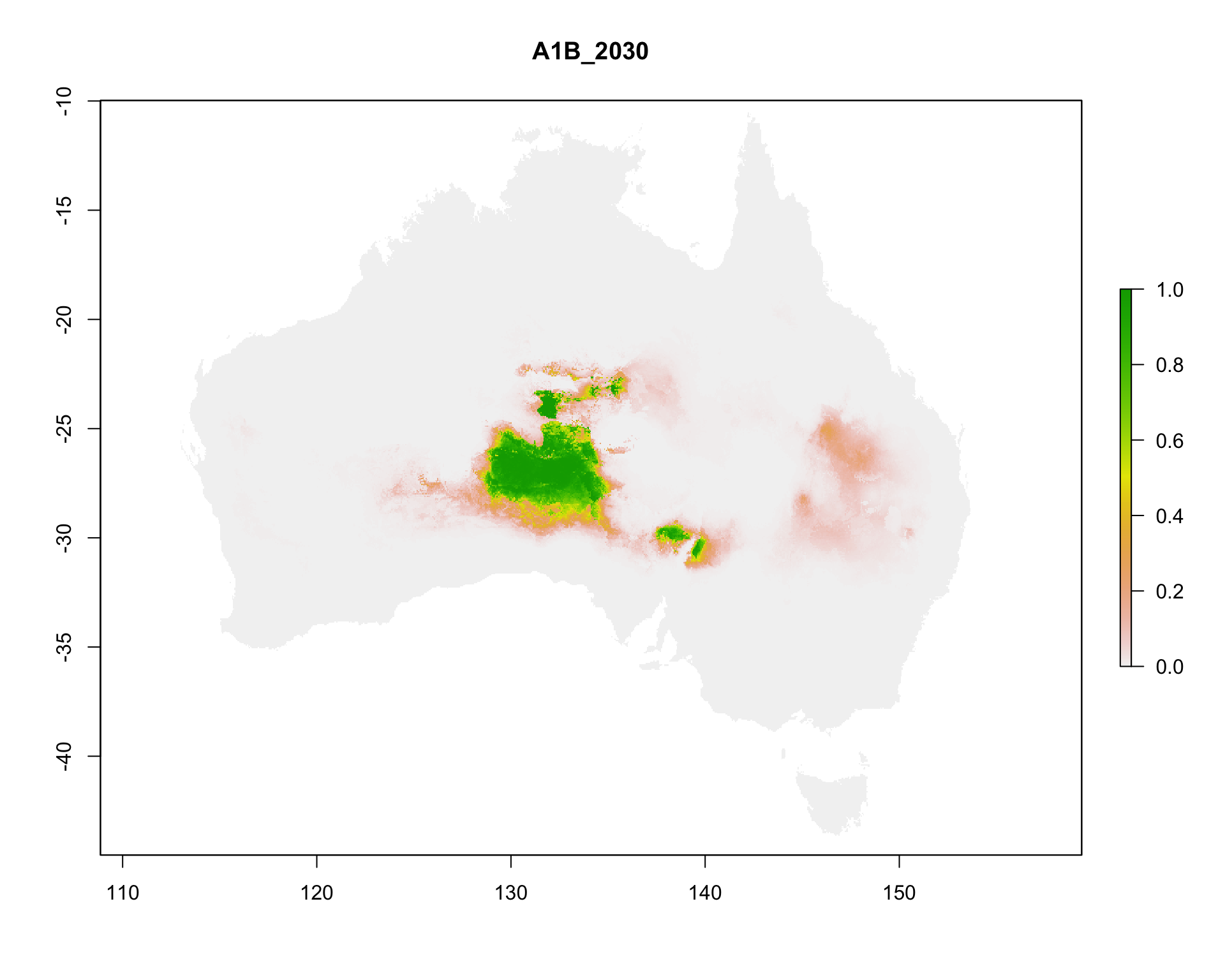
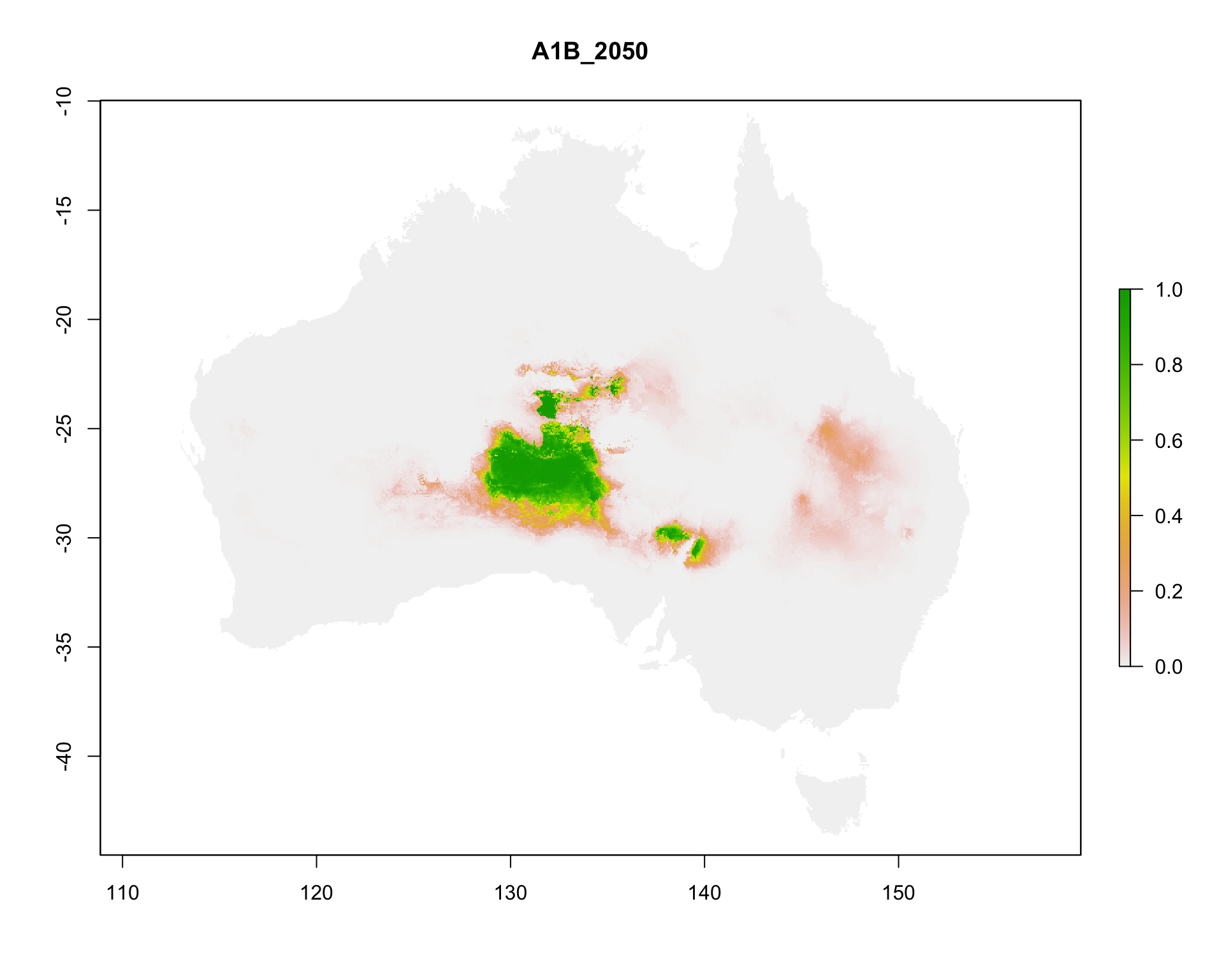
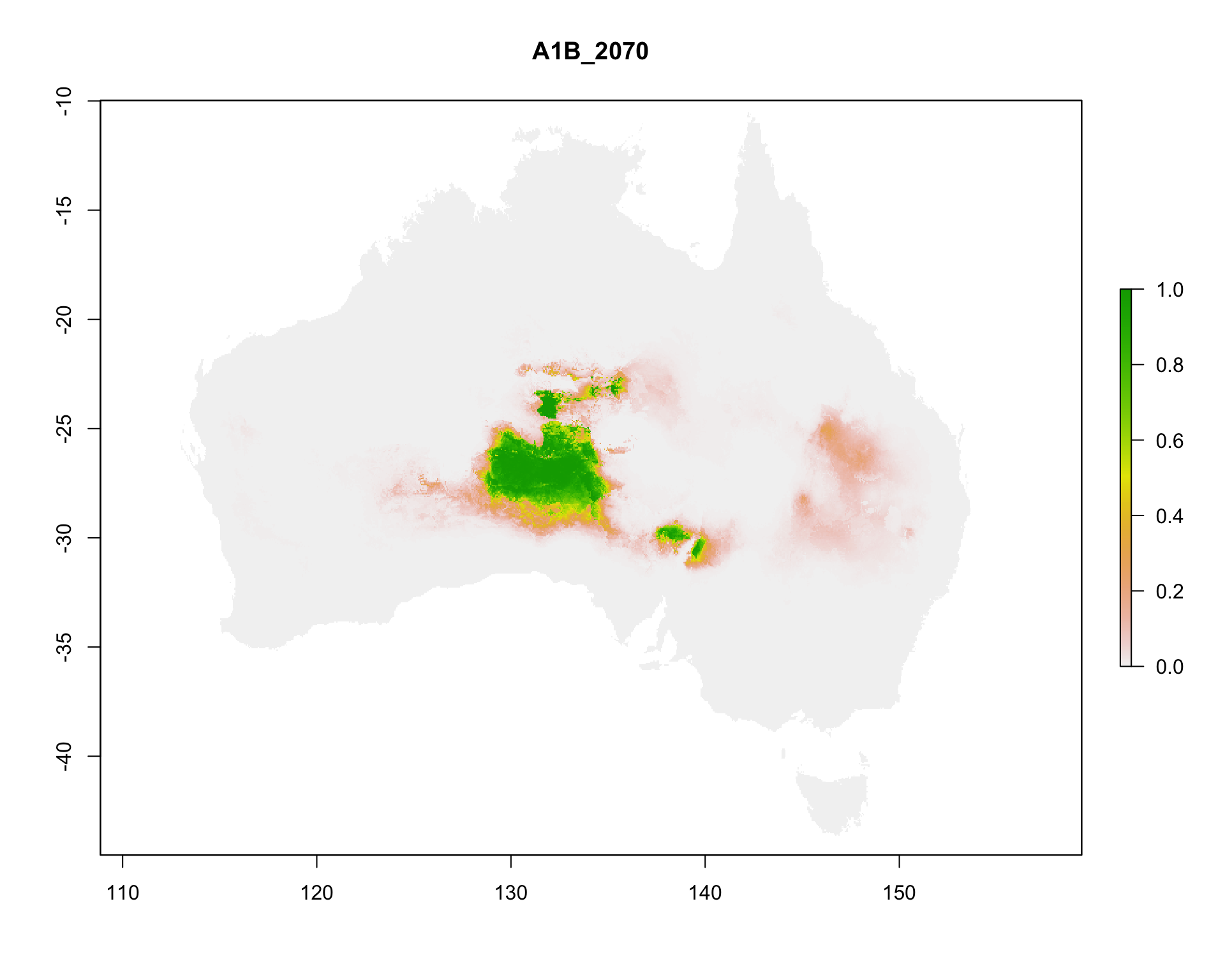
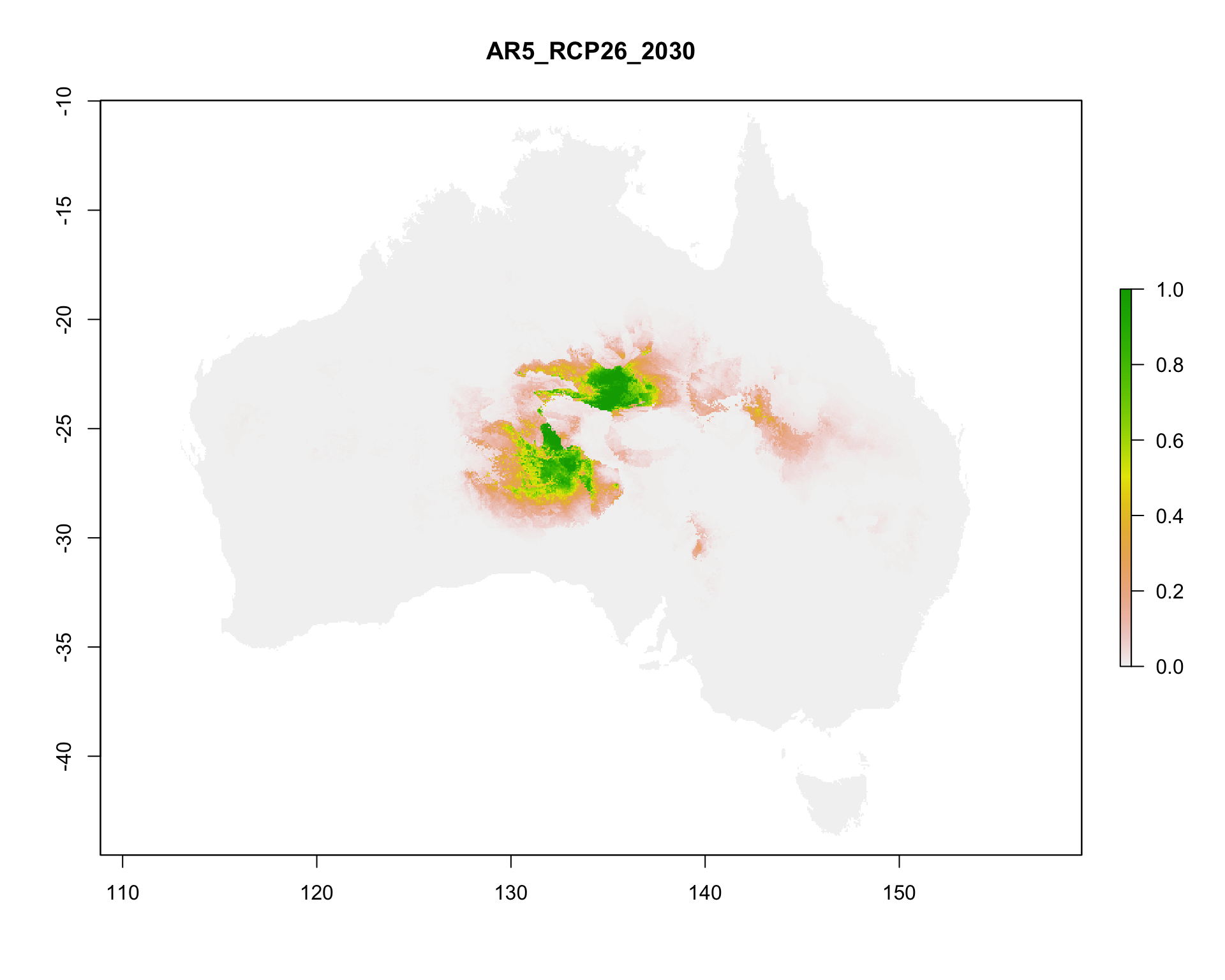
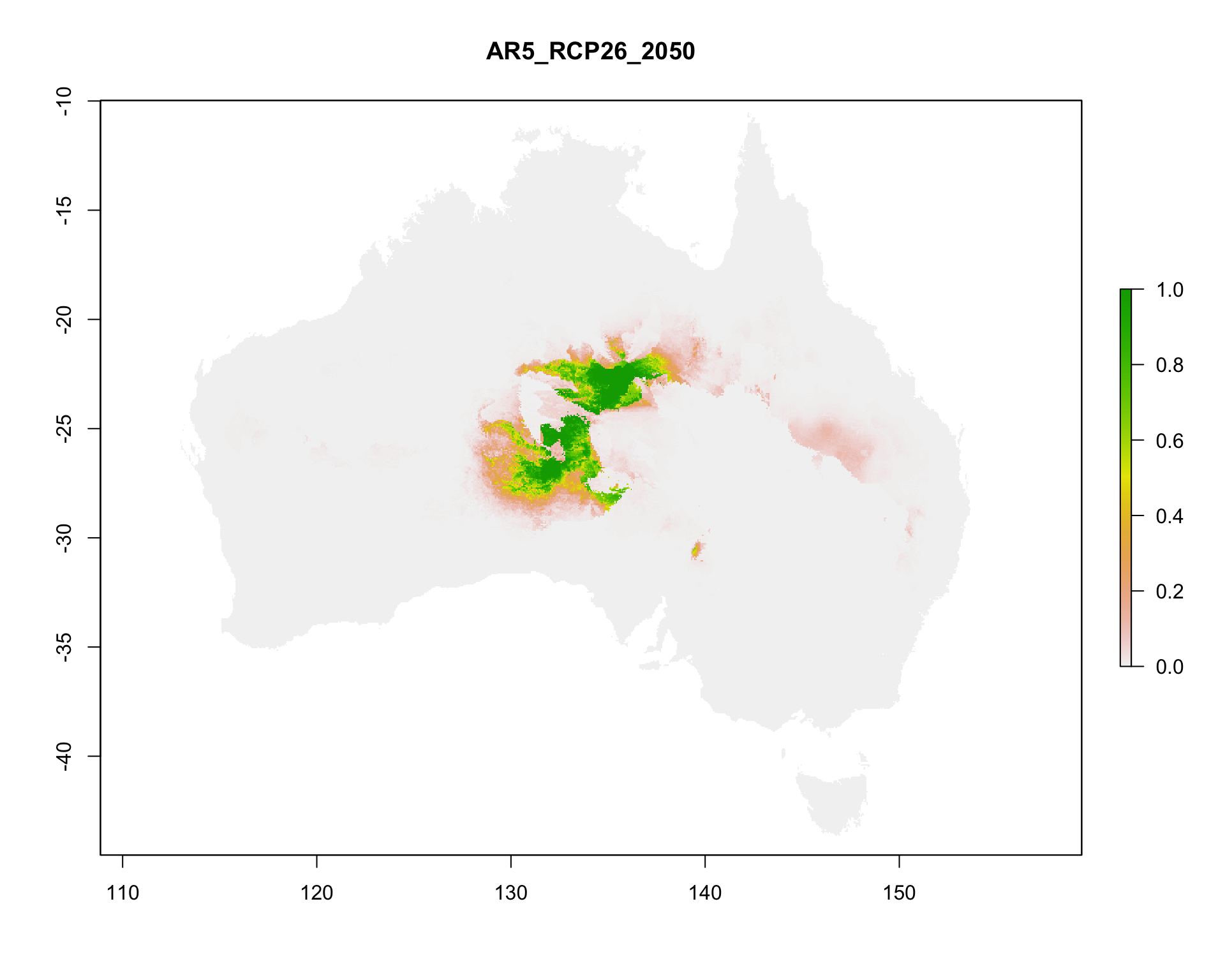
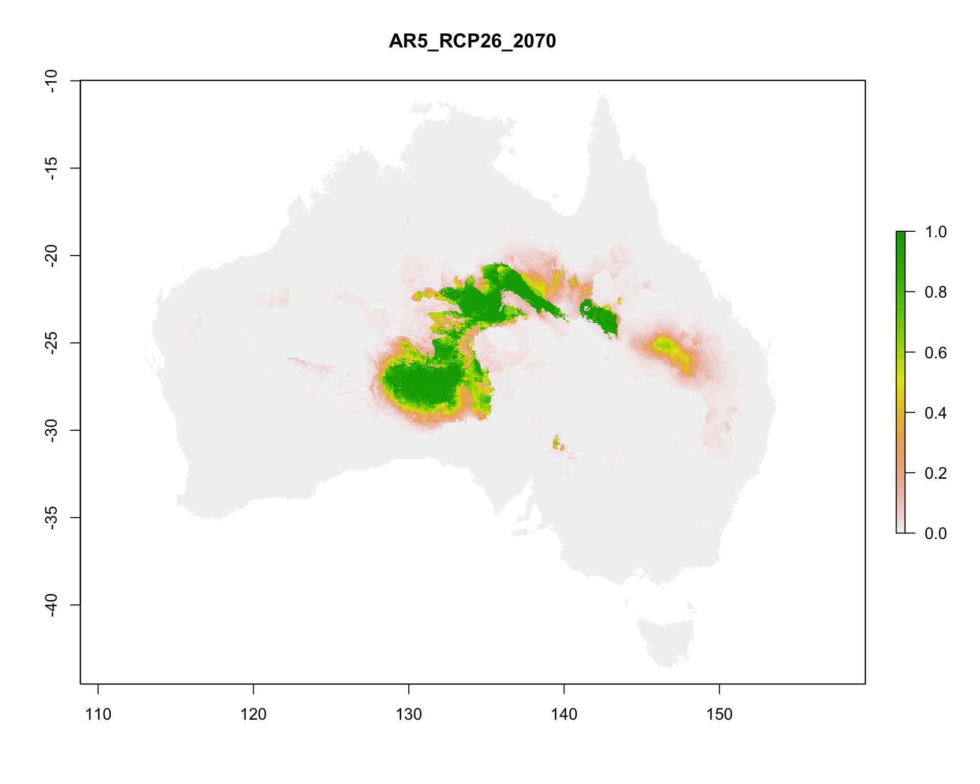
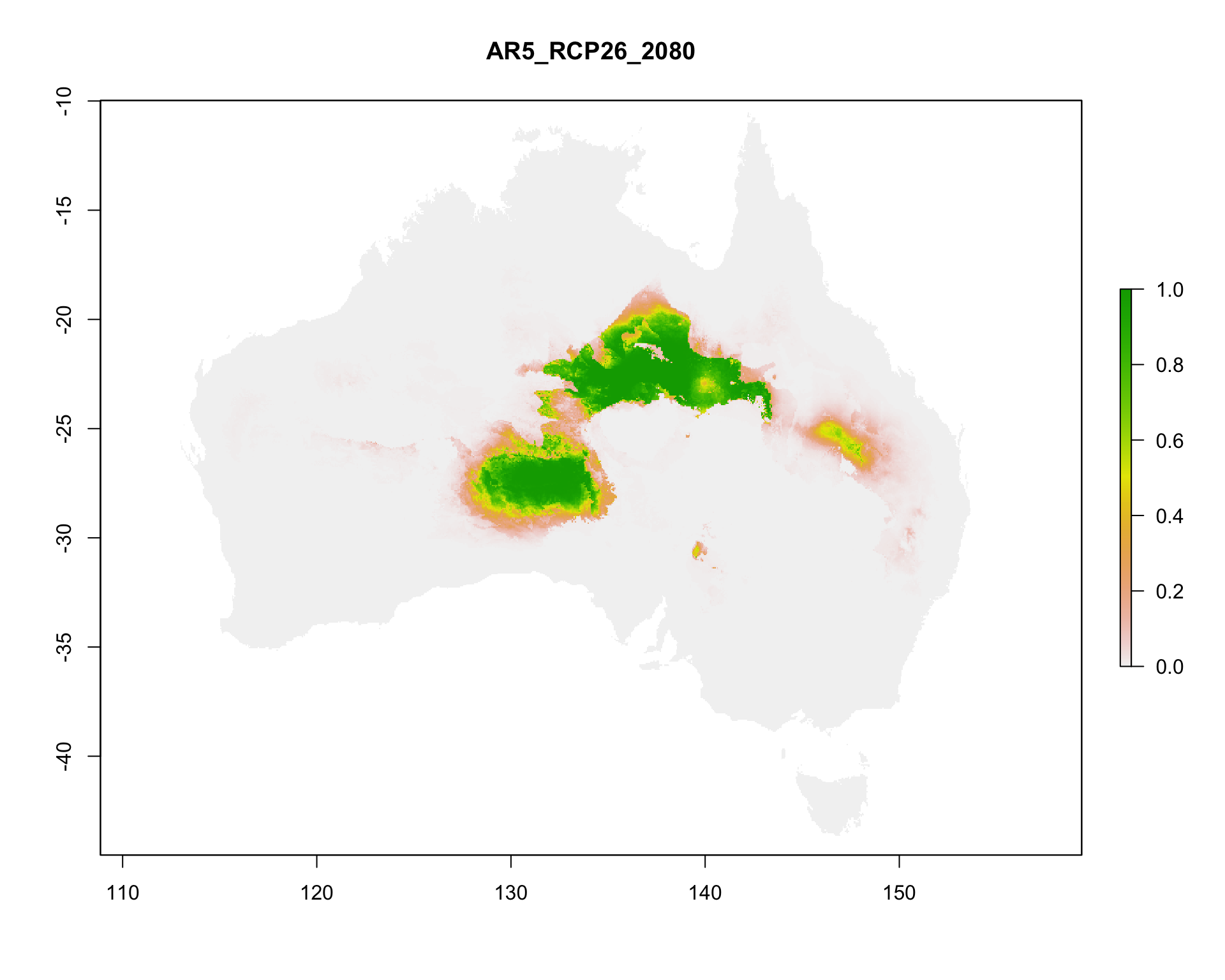
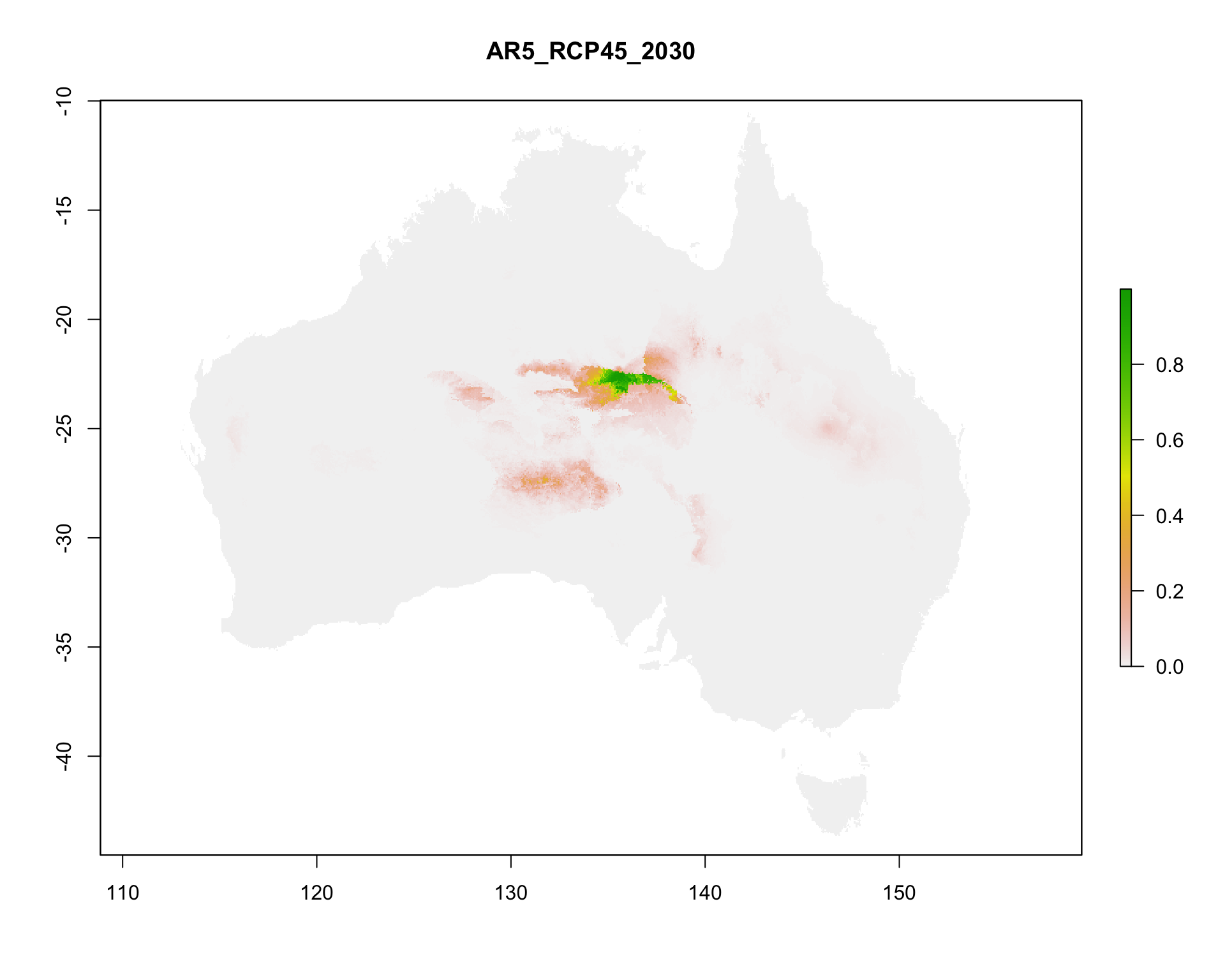
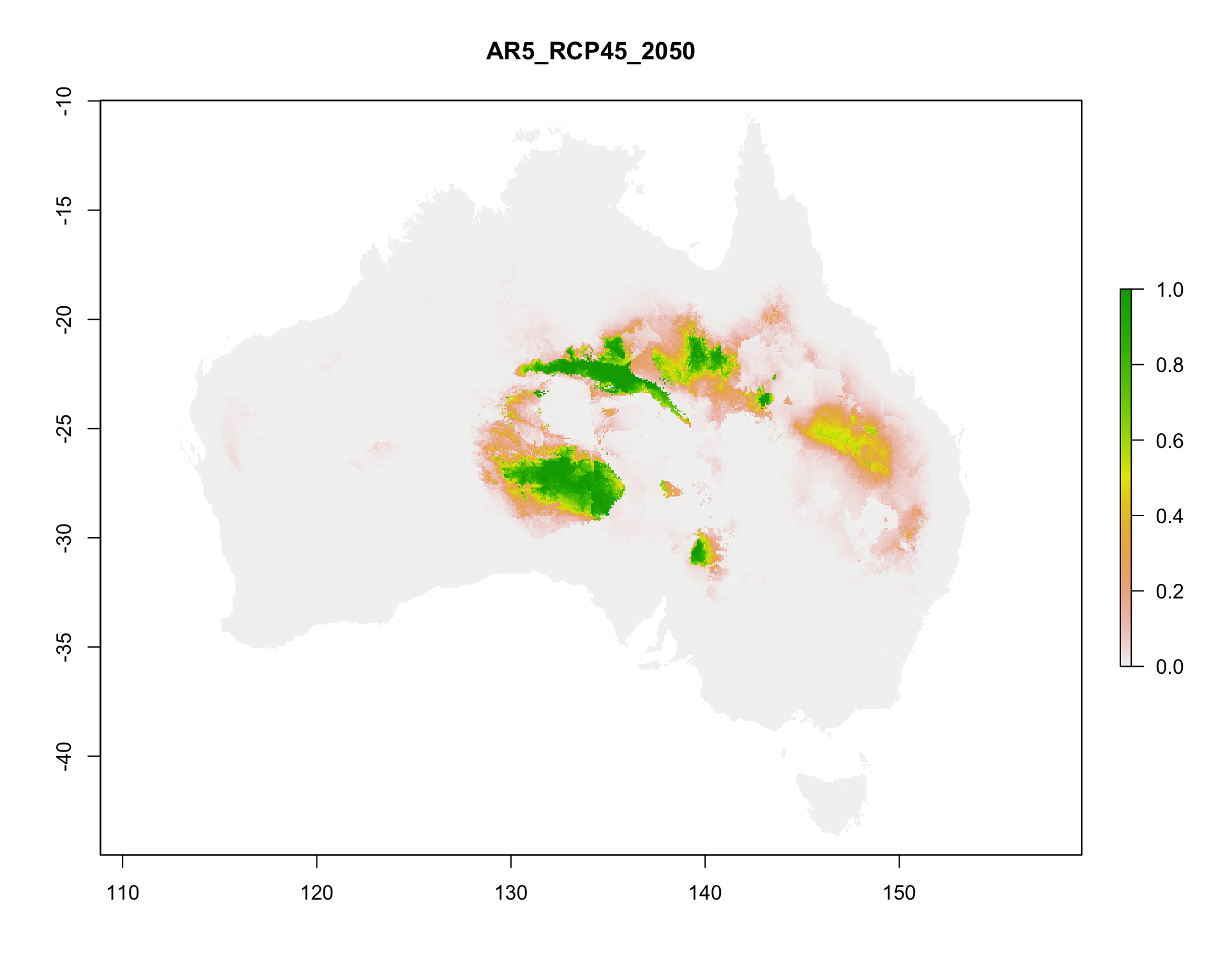
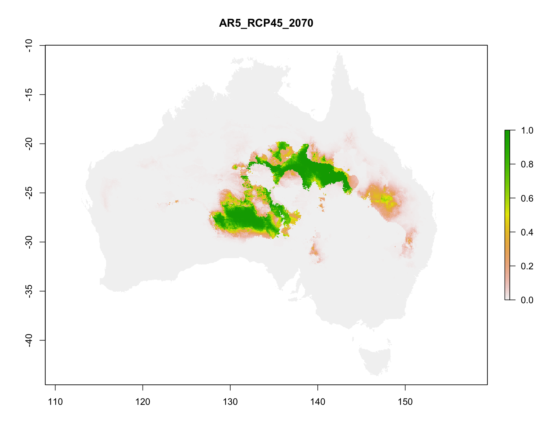
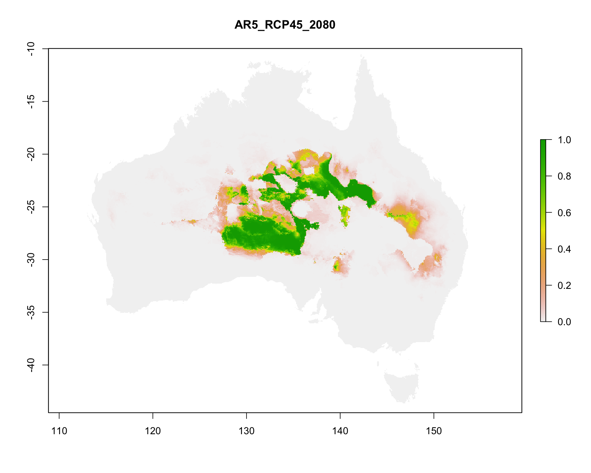
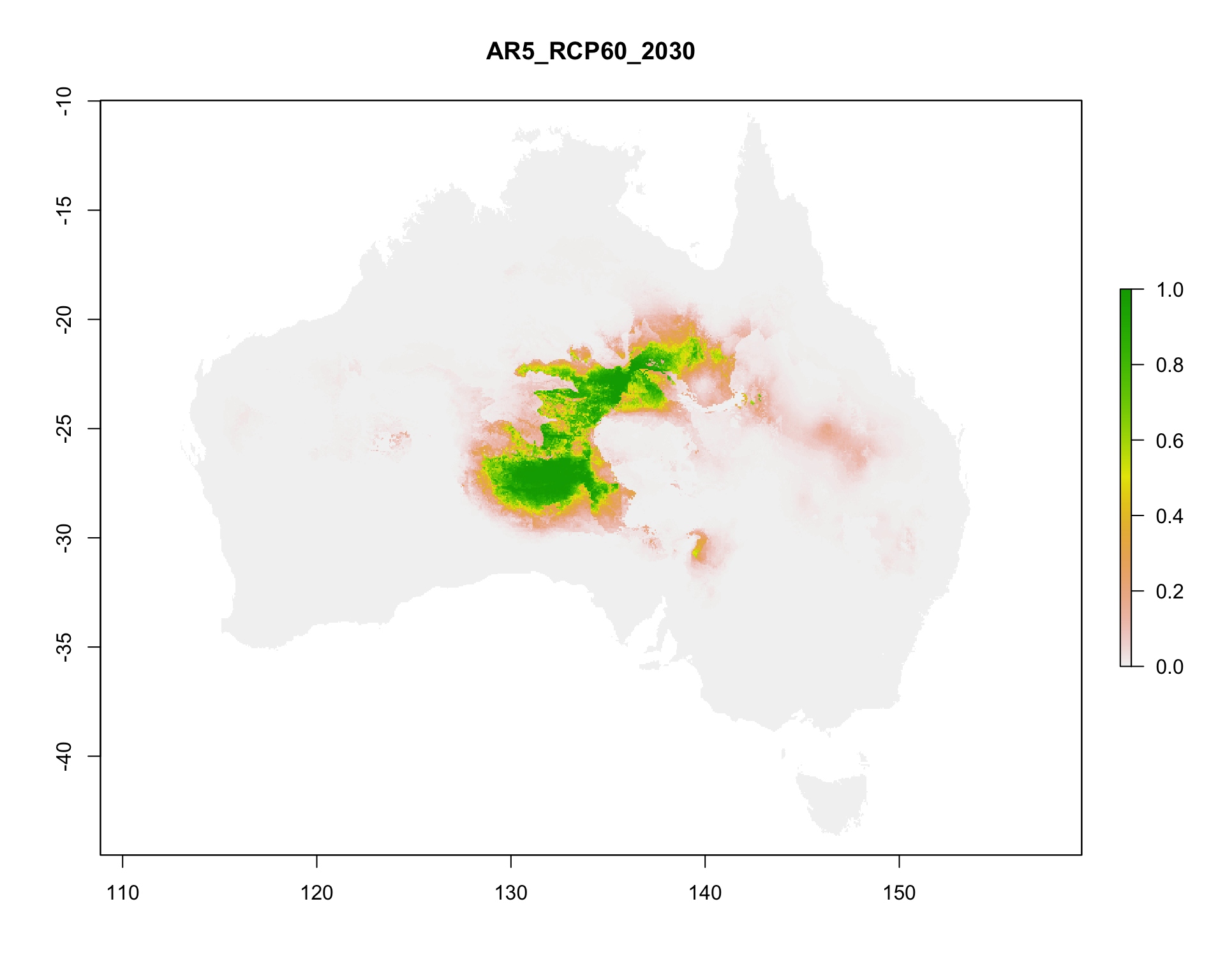
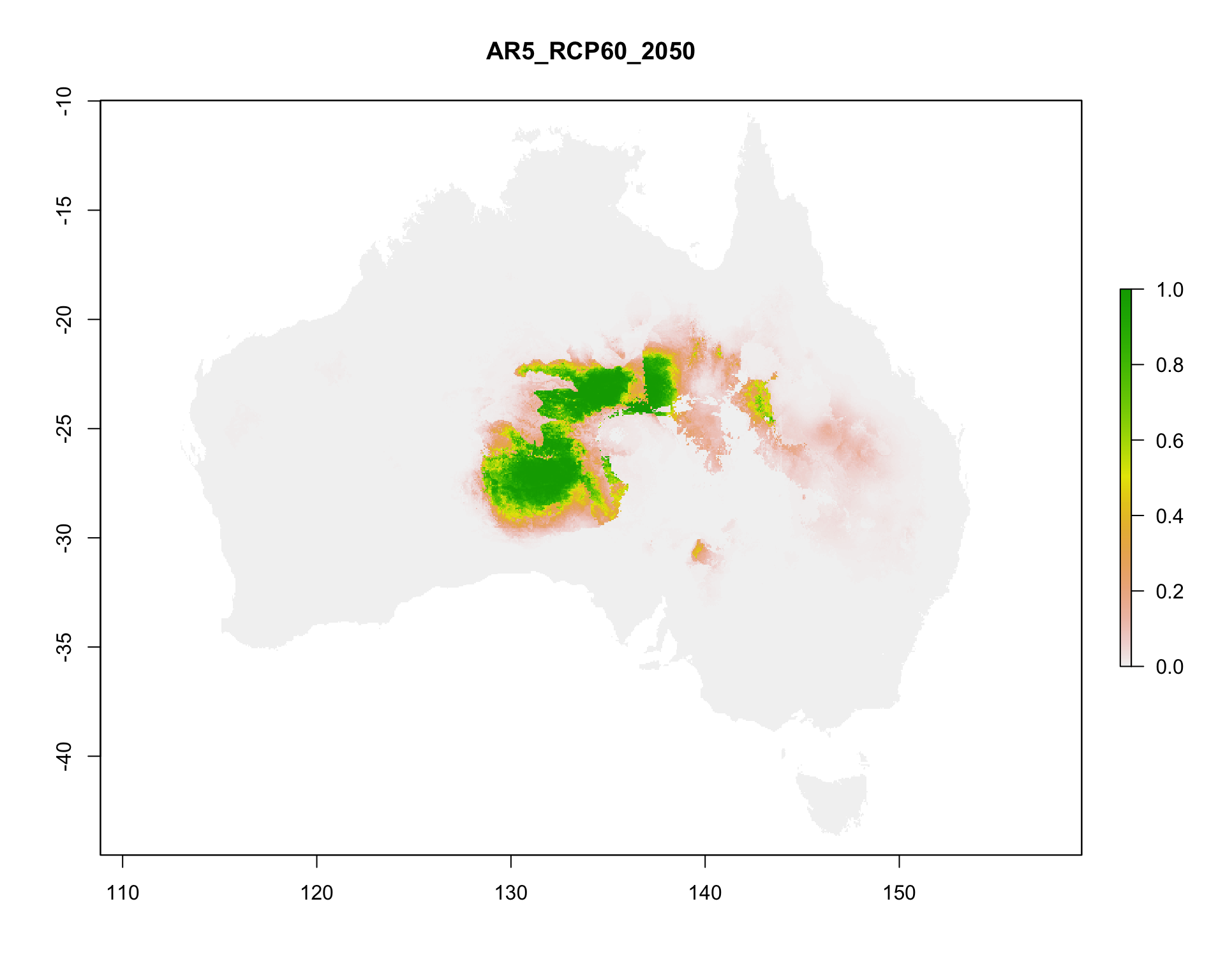
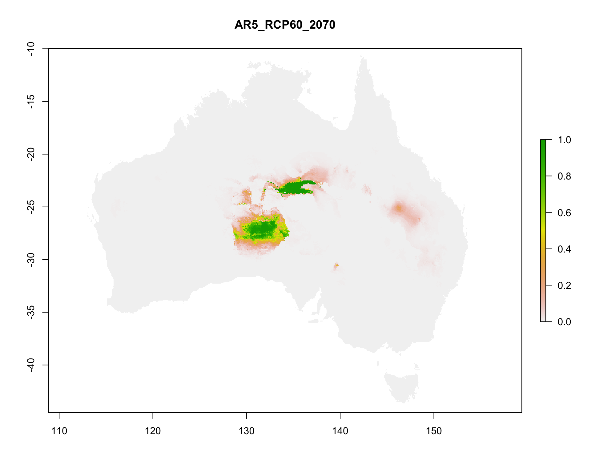
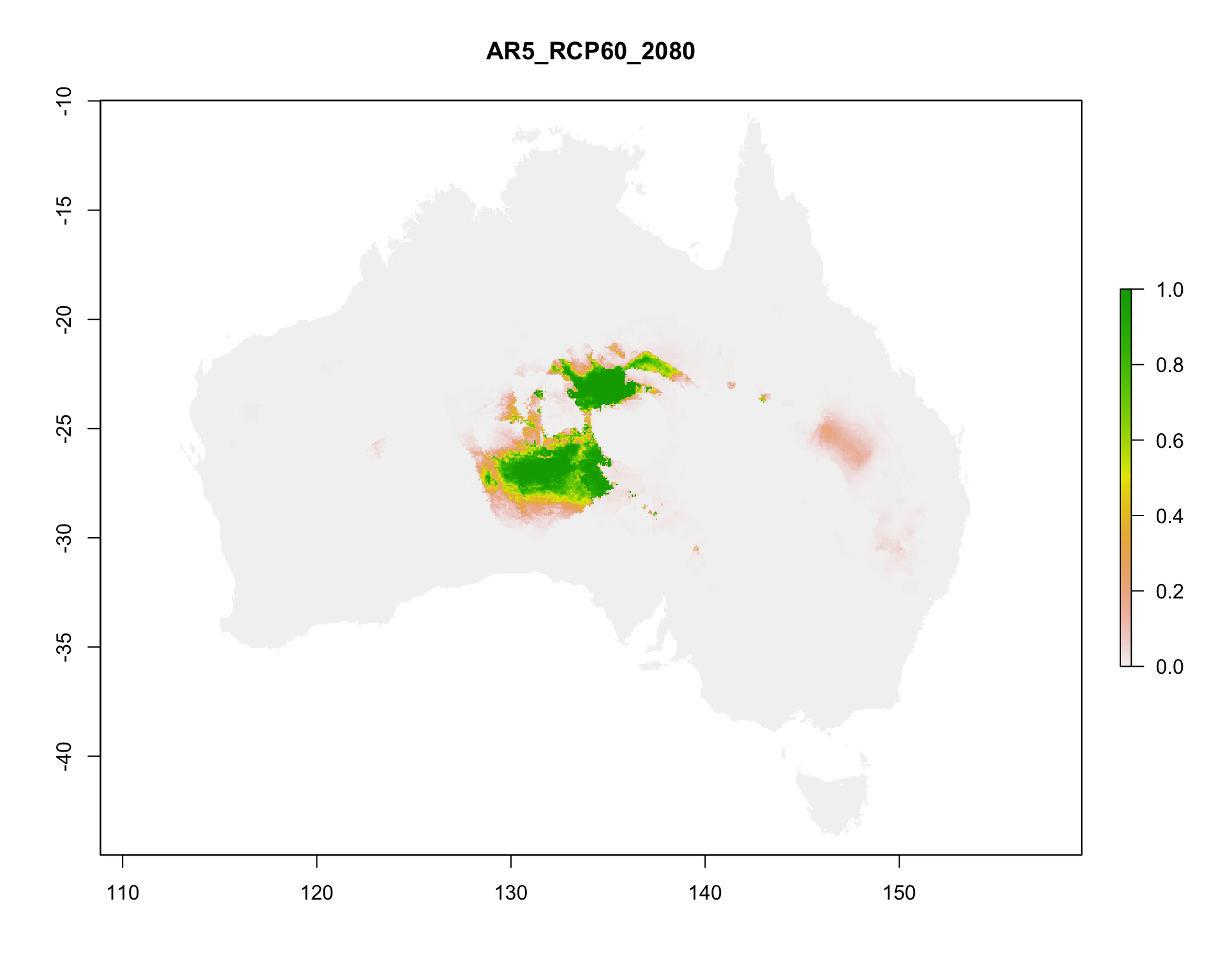
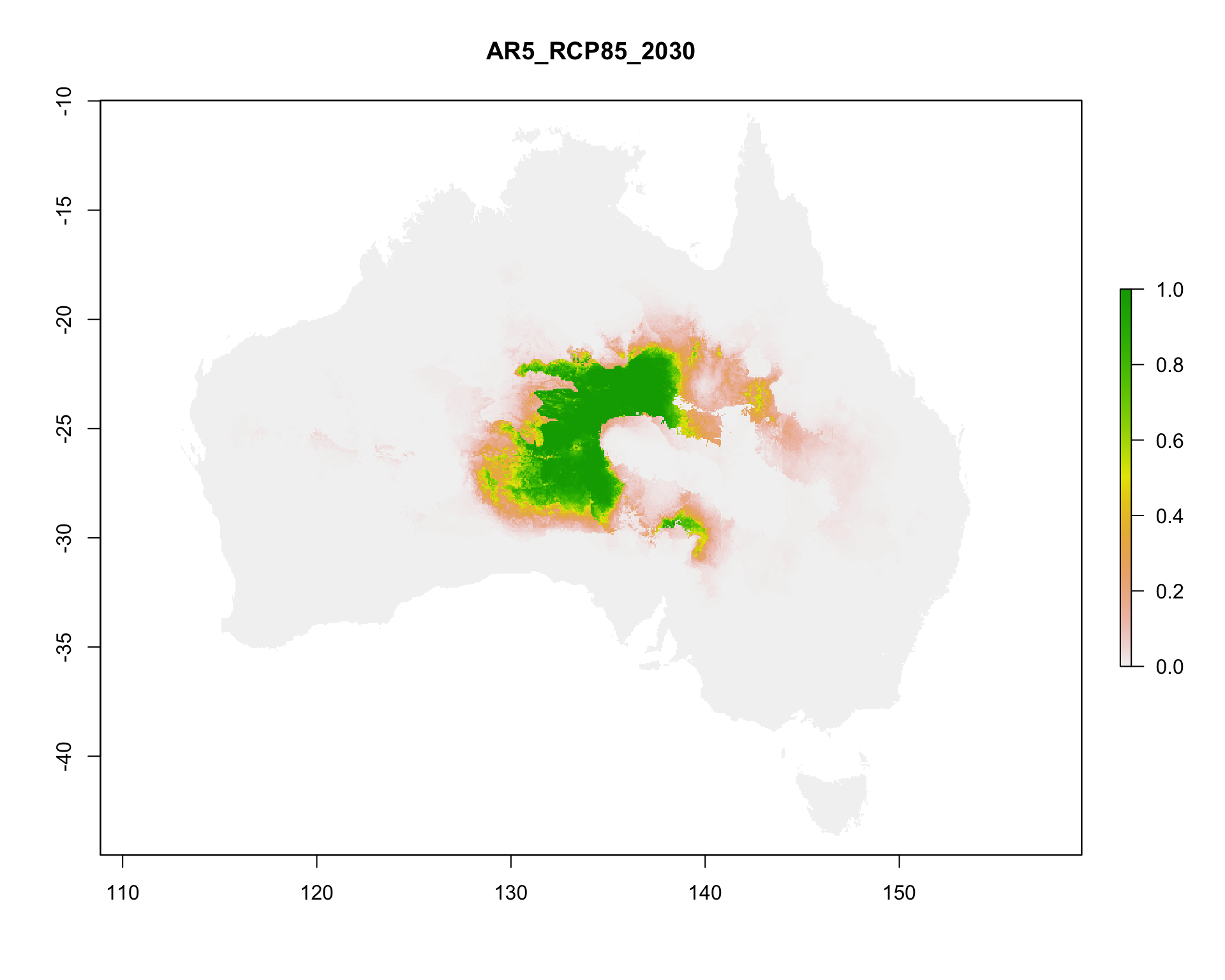
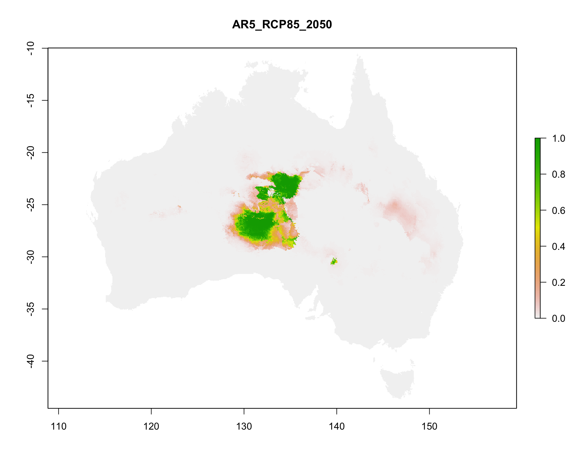
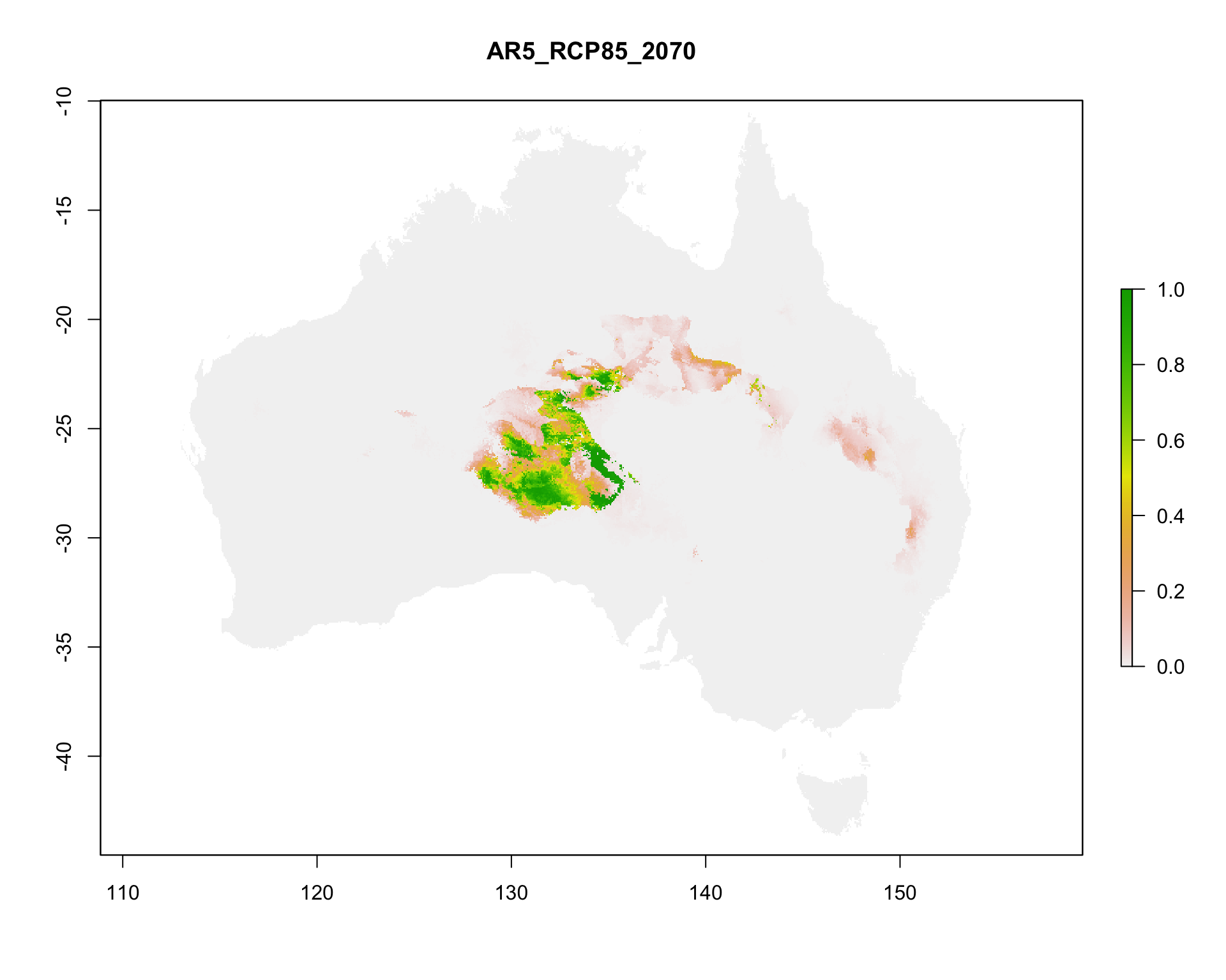
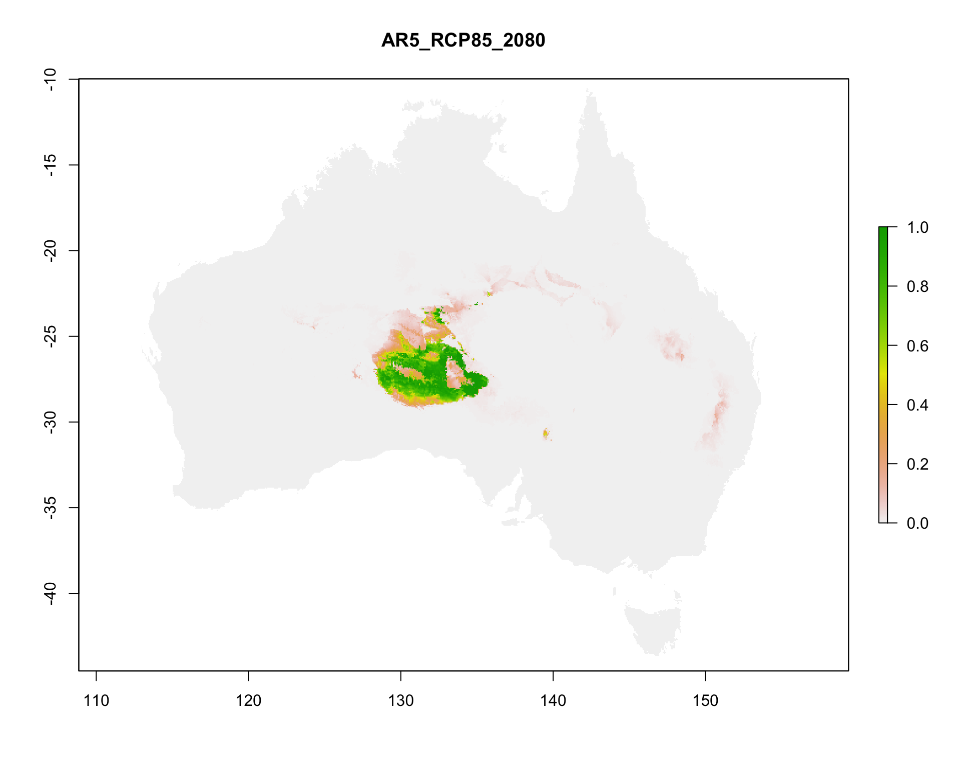
4. Project the model to 19 future climate scenarios from CSIRO Mk3.6: SRES A1B for 2030, 2050 and 2070, and RCP 2.6, 4.5, 6.0 and 8.5 for 2030, 2050, 2070 and 2080.
5. Combine the results with the documented evidence from the 2015 assessment and assign IUCN categories.
6. Compare the result with the published assessment [@Wardle_2015].
- **Outputs:** maps, rasters, model files and tables in `results/`; data inventory, parameters, session information and workflow notes in `provenance/`.
- **Requirements:** R with Java (MaxEnt runs through `rJava`), about 8 GB of memory for Java, about 3 GB of free disk space for the downloaded data, and internet access for Step 1. Run time and peak memory are recorded in `provenance/`.
:::{.aside}
To run the workflow, open this file in RStudio and render it, or run `quarto render Gidgee_workflow_2026.qmd` from the repository root. Step 0 installs any missing R packages into your R library.
**TODO: add tested R version and typical run time.**
:::
## Data sources {#data-sources}
All inputs are downloaded in Step 1 from two public archives supplied with TERN CoESRA Case Study 2.
:::{.aside}
- **TODO:** occurrence data download (GBIF / ALA) and climate, soil and IBRA dataset citations from the Data sources table.
:::
| Data | Source | Used for | Licence and attribution |
|--------------|--------------|--------------|-------------------------------|
| *Acacia georginae* occurrence records (272 records before cleaning) | **TODO:** GBIF download DOI and/or Atlas of Living Australia query, with access date | Criterion B; model presences | **TODO:** GBIF and ALA records carry CC0, CC BY 4.0 or CC BY-NC 4.0 per record; cite the download DOI |
| Baseline climate: 19 bioclimatic variables, c. 2000, 0.05° (3 arcmin) | **TODO:** original climate dataset | Model predictors | **TODO** |
| Future climate: CSIRO Mk3.6, SRES A1B and RCP 2.6–8.5 | **TODO:** original climate dataset | Model projections | **TODO** |
| Soil type grid | **TODO:** original dataset | Categorical predictor | **TODO** |
| IBRA bioregion grid | Interim Biogeographic Regionalisation for Australia v7 (Department of the Environment 2012) | Categorical predictor | **TODO:** confirm licence (CC BY expected) |
| Original Kepler / BCCVL workflow files | TERN CoESRA Case Study 2 | Assessor notes for Criteria A, D and E | **TODO** |
The Google Drive links are not persistent identifiers. Before release, the input archives should be deposited with a DOI (for example in Zenodo) and Step 1 updated to download from there.
## Study area and limitations
**Study area.** The case study defines the study area as the union of 13 IBRA7 regions:
| Code | IBRA7 region | Code | IBRA7 region |
|------|----------------------------|------|-------------------------------|
| BRT | Burt Plain | MGD | Mitchell Grass Downs |
| CHC | Channel Country | MII | Mount Isa Inlier |
| DEU | Desert Uplands | MUL | Mulga Lands |
| DMR | Davenport Murchison Ranges | SSD | Simpson Strzelecki Dunefields |
| FIN | Finke | STP | Stony Plains |
| GSD | Great Sandy Desert | TAN | Tanami |
| MAC | MacDonnell Ranges | | |
This workflow does not crop to those regions. The supplied IBRA grid holds numeric codes without a legend, so regions cannot be selected by name. The model therefore uses the full extent of the supplied rasters, which is continental Australia (111.975–156.275° E, 44.525–9.975° S, 0.05° cells), and IBRA bioregion enters the model as a categorical predictor. The continental extent affects the background sample and the suitable-area totals. Cropping to the official study area needs the IBRA7 polygons with their region codes.
**Other limitations.**
- **Criterion A** cannot be calculated: there is no historical time series of the ecosystem's distribution. The projected change in suitable climate (Step 8) is supporting context, not evidence of decline.
- **Criterion B** is assessed from the order of magnitude of EOO and AOO, not checked against the official IUCN threshold table.
- **Criteria D and E** are taken from the 2015 assessors' documented, literature-based notes, preserved in the Kepler workflow, not recalculated.
- **AR5 2080 layers** were supplied at 2.5 arcmin instead of 3 arcmin and are bilinearly resampled to the baseline grid; these rows are flagged `resampled = TRUE` in `future_suitability_change.csv`.
- **Model settings:** a single MaxEnt run with automatic feature types and regularisation multiplier 1; no cross-validation replicates.
- **Software:** `raster` and `dismo` are superseded by `terra` and `predicts`. Package versions are recorded in `provenance/` rather than pinned with `renv`.
## Session setup
Starts the run timer and configures Java (8 GB memory, headless mode) before MaxEnt loads.
```{r}
#| label: Session setup
# Record the complete script runtime from the first executable step.
t_start <- Sys.time()

# Reset R's memory-usage counters here too, so the peak-memory figure
# recorded in Step 12 covers the whole run, not just whatever ran since the
# last garbage collection. gc()'s "max used" tracks R's own heap only — it
# does not see the separate JVM heap dismo::maxent() allocates via rJava
# (capped at -Xmx8g below); Step 12 notes that caveat next to the number.
gc(reset = TRUE)
# Allocate Java memory, force headless mode, and set an explicit JVM thread
# stack size before rJava, raster or dismo can start the JVM.
# -Djava.awt.headless=true stops MaxEnt from trying to open a Swing/AWT
# progress window (which cannot render in this context and crashes the JVM).
# -Xss2560k works around a known RStudio-Desktop-on-macOS issue where
# RStudio launches R with a smaller default thread stack than plain
# command-line R, which crashes the JVM outright at initialisation
# ("R Session Aborted" right at "Loading required namespace: rJava").
# NOAWT further disables AWT-dependent code paths some Java packages check.
Sys.setenv(NOAWT = TRUE)
options(java.parameters = c("-Xmx8g", "-Xss2560k", "-Djava.awt.headless=true"))
```
## Project folders
Defines the project folders relative to the working directory and creates them if needed.
```{r}
#| label: Setup
# Configuration ---------------------------------------------------------------
# Use the directory from which this script/notebook is being run as the
# project directory. This avoids using the old CoESRA file paths.
project_dir <- normalizePath(getwd(), winslash = "/", mustWork = TRUE)
setwd(project_dir)

# Define project folders used by this stage of the workflow.
raw_dir <- file.path(project_dir, "data", "raw")
processed_dir <- file.path(project_dir, "data", "processed")
provenance_dir <- file.path(project_dir, "provenance")
results_dir <- file.path(project_dir, "results")
results_maps_dir <- file.path(results_dir, "maps")
results_spatial_dir <- file.path(results_dir, "spatial")
results_models_dir <- file.path(results_dir, "models")
results_models_baseline_dir <- file.path(results_models_dir, "baseline")
results_models_a1b_dir <- file.path(results_models_dir, "A1B")
results_models_ar5_dir <- file.path(results_models_dir, "AR5")
results_future_maps_dir <- file.path(results_maps_dir, "future_suitability_maps")
results_tables_dir <- file.path(results_dir, "tables")

# Create folders if they do not already exist.
dir.create(raw_dir, recursive = TRUE, showWarnings = FALSE)
dir.create(processed_dir, recursive = TRUE, showWarnings = FALSE)
dir.create(provenance_dir, recursive = TRUE, showWarnings = FALSE)
dir.create(results_maps_dir, recursive = TRUE, showWarnings = FALSE)
dir.create(results_spatial_dir, recursive = TRUE, showWarnings = FALSE)
dir.create(results_models_baseline_dir, recursive = TRUE, showWarnings = FALSE)
dir.create(results_models_a1b_dir, recursive = TRUE, showWarnings = FALSE)
dir.create(results_models_ar5_dir, recursive = TRUE, showWarnings = FALSE)
dir.create(results_future_maps_dir, recursive = TRUE, showWarnings = FALSE)
dir.create(results_tables_dir, recursive = TRUE, showWarnings = FALSE)
```
## Step 0: Requirements
Installs any missing R packages and loads them.
```{r}
#| label: Step 0 Requirements
options(repos = c(CRAN = "https://cloud.r-project.org"))

required_packages <- c(
  "googledrive", # Downloads the public Google Drive files.
  "fs",          # Creates and checks project file paths.
  "digest",      # Calculates SHA-256 file fingerprints.
  "sessioninfo", # Records detailed R session information.
  "readr",       # Reads tabular input data.
  "dplyr",       # Provides data transformation functions.
  "raster",      # Handles raster environmental data.
  "sf",          # Handles coordinate reference systems and projections.
  "xml2",        # Parses the preserved Kepler workflow XML for Step 9.
  "dismo",       # Supports habitat suitability modelling.
  "maps",        # Provides geographic map data.
  "leaflet",     # Provides interactive map outputs.
  "rJava"        # Provides low-Level R to Java Interface
)

is_installed <- function(pkg) nzchar(system.file(package = pkg))
missing_packages <- required_packages[!vapply(required_packages, is_installed, logical(1))]

if (length(missing_packages) > 0) {
  install.packages(missing_packages)
}

library(googledrive)
library(fs)
library(digest)
library(sessioninfo)
library(readr)
library(dplyr)
library(raster)
library(sf)
library(xml2)
library(dismo)
library(maps)
library(leaflet)
```
## Step 1: Get data
Downloads the two public case-study archives from Google Drive (no login required), extracts them into `data/raw/`, and records an inventory of every file with its SHA-256 checksum for provenance.
```{r}
#| label: Step 1 Get data
# Public file identifiers -----------------------------------------------------
# These IDs come from the public links supplied for Case 2.
public_files <- data.frame(
  id = c(
    "1CnpAGCjvHVkS2BfOmVDVbjSQ8JvoS-_9",
    "1F7KNVAQ2RXPC09m1xV_E8gNujjmGom1s"
  ),
  output_name = c(
    "gidgee_data_and_scripts",
    "gidgee_workflow_files"
  ),
  source_url = c(
    "https://drive.google.com/file/d/1CnpAGCjvHVkS2BfOmVDVbjSQ8JvoS-_9/view?usp=sharing",
    "https://drive.google.com/file/d/1F7KNVAQ2RXPC09m1xV_E8gNujjmGom1s/view?usp=sharing"
  ),
  stringsAsFactors = FALSE
)

# Download public files without using a personal Google account.
drive_deauth()

# Download each public file to data/raw/.
for (i in seq_len(nrow(public_files))) {
  destination <- file.path(raw_dir, public_files$output_name[i])

  drive_download(
    file = as_id(public_files$id[i]),
    path = destination,
    overwrite = TRUE
  )
}
# Unzip downloaded archives -----------------------------------------------------
# Extract each downloaded file if it is actually a zip archive; otherwise
# leave it as-is. Extraction goes into a sibling folder so the original
# downloaded archive is preserved unchanged.
unzip_if_archive <- function(path) {
  contents <- tryCatch(
    utils::unzip(path, list = TRUE),
    error = function(e) NULL
  )

  if (is.null(contents)) {
    return(invisible(FALSE))
  }

  extract_dir <- paste0(path, "_extracted")
  dir.create(extract_dir, recursive = TRUE, showWarnings = FALSE)
  utils::unzip(path, exdir = extract_dir, overwrite = TRUE)
  invisible(TRUE)
}

for (i in seq_len(nrow(public_files))) {
  destination <- file.path(raw_dir, public_files$output_name[i])
  unzip_if_archive(destination)
}

# Load/check downloaded files -------------------------------------------------
# Create an inventory showing each file's path, size and SHA-256 checksum.
# A SHA-256 checksum is a digital fingerprint used to detect file changes.
input_files <- fs::dir_ls(raw_dir, type = "file", recurse = TRUE)

input_inventory <- data.frame(
  file = unname(as.character(input_files)),
  size_bytes = unname(as.numeric(fs::file_size(input_files))),
  sha256 = unname(vapply(
    input_files,
    digest,
    character(1),
    file = TRUE,
    algo = "sha256"
  )),
  row.names = NULL,
  stringsAsFactors = FALSE
)

# Print a short summary rather than dumping every row (800+ files) to console;
# the full inventory is still written out below.
cat("Files inventoried:", nrow(input_inventory), "\n")
cat("Total size (MB):", round(sum(input_inventory$size_bytes) / 1e6, 1), "\n")
# Record the inventory for provenance.
write.csv(
  input_inventory,
  file.path(provenance_dir, "input_inventory.csv"),
  row.names = FALSE
)
```
## Step 2: Inspect the downloaded files
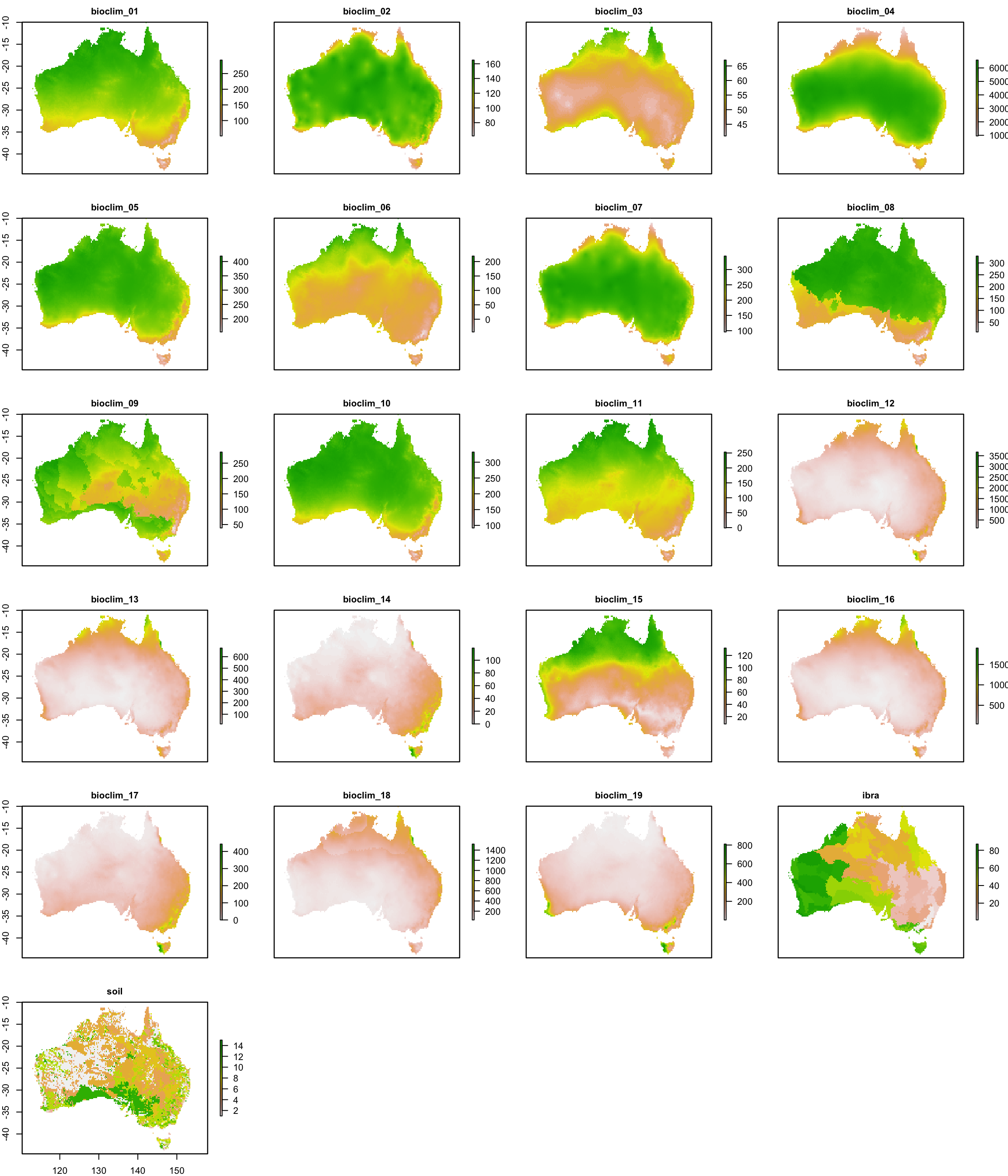
Identifies the occurrence CSV, the baseline, A1B and AR5 climate layers and the original Kepler workflow files, then plots every baseline layer to confirm it is readable.
```{r}
#| label: Step 2 Inspect the downloaded files
#| fig-width: 12
#| fig-height: 14
# List all extracted files -----------------------------------------------------
# Exclude the original ZIP archives and macOS zip metadata (__MACOSX).
extracted_files <- fs::dir_ls(raw_dir, type = "file", recurse = TRUE)
extracted_files <- extracted_files[grepl("_extracted/", extracted_files)]
extracted_files <- extracted_files[!grepl("__MACOSX", extracted_files)]

# Identify the occurrence CSV ---------------------------------------------------
occurrence_csv <- extracted_files[grepl("SpeciesOccurence_clean\\.csv$", extracted_files)]
stopifnot("Occurrence CSV not found" = length(occurrence_csv) == 1)

# Identify climate/environmental layers -----------------------------------------
# Each layer is stored as an ESRI ASCII grid (.asc) with a matching .prj file.
climate_layers <- extracted_files[grepl("\\.asc$", extracted_files)]

# Identify scripts and workflow files -------------------------------------------
script_files <- extracted_files[
  grepl("\\.(sh|R|py)$", extracted_files, ignore.case = TRUE) |
    grepl("/bccvl/", extracted_files)
]

# Identify baseline, A1B and AR5 folders -----------------------------------------
baseline_dir <- unique(dirname(climate_layers[grepl("/Baseline/", climate_layers)]))
a1b_dir      <- unique(dirname(climate_layers[grepl("/A1B/", climate_layers)]))
ar5_dir      <- unique(dirname(climate_layers[grepl("/AR5/", climate_layers)]))

# Confirm the original Kepler XML files are preserved for provenance ------------
kepler_xml_files <- extracted_files[grepl("\\.xml$", extracted_files, ignore.case = TRUE)]

# Summary ------------------------------------------------------------------------
inspection_summary <- data.frame(
  category = c(
    "Occurrence CSV",
    "Climate/environmental layers (.asc)",
    "Script/workflow files",
    "Baseline scenario folders",
    "A1B scenario folders",
    "AR5 scenario folders",
    "Kepler XML files"
  ),
  count = c(
    length(occurrence_csv),
    length(climate_layers),
    length(script_files),
    length(baseline_dir),
    length(a1b_dir),
    length(ar5_dir),
    length(kepler_xml_files)
  )
)

print(inspection_summary)
stopifnot(
  "No baseline climate layers found" = length(baseline_dir) > 0,
  "No A1B climate layers found" = length(a1b_dir) > 0,
  "No AR5 climate layers found" = length(ar5_dir) > 0,
  "Kepler XML files missing" = length(kepler_xml_files) > 0
)

# View all baseline raster layers -------------------------------------------------
# Load every baseline layer as a raster stack and plot them together to
# visually confirm the environmental layers are readable before they are
# used in later steps.
baseline_layer_paths <- fs::dir_ls(baseline_dir[1], glob = "*.asc")
baseline_stack <- raster::stack(baseline_layer_paths)

# Use clean layer names instead of full file paths for the panel titles.
names(baseline_stack) <- tools::file_path_sans_ext(basename(baseline_layer_paths))

print(baseline_stack)
raster::plot(
  baseline_stack,
  col = rev(terrain.colors(255)),
  nc = 4,
  maxnl = raster::nlayers(baseline_stack),
  cex.main = 1
)
```
## Step 3: Load and validate occurrence data
Checks the coordinates for missing values, duplicates and points outside mainland Australia, removes invalid records and saves the cleaned table.
```{r}
#| label: Step 3 Load and validate occurrence data
# Load the occurrence CSV ---------------------------------------------------------
occurrences_raw <- readr::read_csv(occurrence_csv, show_col_types = FALSE)

# Inspect column names and data types ----------------------------------------------
dplyr::glimpse(occurrences_raw)
# Check latitude and longitude fields ------------------------------------------------
stopifnot(
  "Longitude column missing" = "Longitude" %in% names(occurrences_raw),
  "Latitude column missing"  = "Latitude" %in% names(occurrences_raw)
)

# Count missing coordinates ----------------------------------------------------------
n_missing_coords <- sum(is.na(occurrences_raw$Longitude) | is.na(occurrences_raw$Latitude))

# Check duplicate records --------------------------------------------------------------
n_duplicate_records <- sum(duplicated(occurrences_raw))

# Check coordinate ranges (mainland Australia bounding box) ----------------------------
valid_lon_range <- c(112, 154)
valid_lat_range <- c(-44, -10)

out_of_range <- with(
  occurrences_raw,
  is.na(Longitude) | is.na(Latitude) |
    Longitude < valid_lon_range[1] | Longitude > valid_lon_range[2] |
    Latitude  < valid_lat_range[1] | Latitude  > valid_lat_range[2]
)
n_out_of_range <- sum(out_of_range)

# Remove invalid or incomplete records ---------------------------------------------------
occurrences_clean <- occurrences_raw[!out_of_range, ]

# Validation summary -----------------------------------------------------------------------
occurrence_validation <- data.frame(
  check = c(
    "Total records",
    "Missing coordinates",
    "Duplicate records",
    "Out-of-range coordinates",
    "Records retained after cleaning"
  ),
  value = c(
    nrow(occurrences_raw),
    n_missing_coords,
    n_duplicate_records,
    n_out_of_range,
    nrow(occurrences_clean)
  )
)

print(occurrence_validation)
# Save the cleaned occurrence table -----------------------------------------------------
readr::write_csv(occurrences_clean, file.path(processed_dir, "occurrences_clean.csv"))
readr::write_csv(occurrence_validation, file.path(provenance_dir, "occurrence_validation.csv"))
```
## Step 4: Define the analysis projection
Projects the occurrence points from WGS84 to GDA94 / Australian Albers (EPSG:3577), so the area calculations in Step 5 use true 10 × 10 km cells.
```{r}
#| label: Step 4 Define the analysis projection
# Read the occurrence coordinates -----------------------------------------------------
# The occurrence CSV and the baseline .asc rasters are both supplied in
# geographic WGS84 (decimal degrees) — confirmed from the rasters' .prj files.
occurrence_points_wgs84 <- sf::st_as_sf(
  occurrences_clean,
  coords = c("Longitude", "Latitude"),
  crs = 4326,
  remove = FALSE
)

# Define the Australian Albers projection used by the original workflow ---------------
# GDA94 / Australian Albers Equal Area (EPSG:3577) is the standard equal-area
# projection used for Australian environmental analyses, needed so that the
# AOO grid cells (Step 5) represent true 10 x 10 km squares on the ground.
analysis_crs <- sf::st_crs(3577)

# Convert longitude/latitude to projected coordinates ----------------------------------
occurrence_points_albers <- sf::st_transform(occurrence_points_wgs84, analysis_crs)
projected_coords <- sf::st_coordinates(occurrence_points_albers)

# Check that the projected points are valid ---------------------------------------------
stopifnot(
  "Projected point count does not match input" =
    nrow(projected_coords) == nrow(occurrences_clean),
  "Projected coordinates contain missing values" =
    !anyNA(projected_coords)
)

# Record the CRS and cell size -----------------------------------------------------------
# 10,000 metre cell size supports the 10 x 10 km AOO grid used in Step 5.
aoo_cell_size_m <- 10000

cat("Analysis CRS:", analysis_crs$input, "\n")
cat("AOO cell size (m):", aoo_cell_size_m, "\n")
print(head(projected_coords))
```
## Step 5: Calculate Criterion B spatial indicators
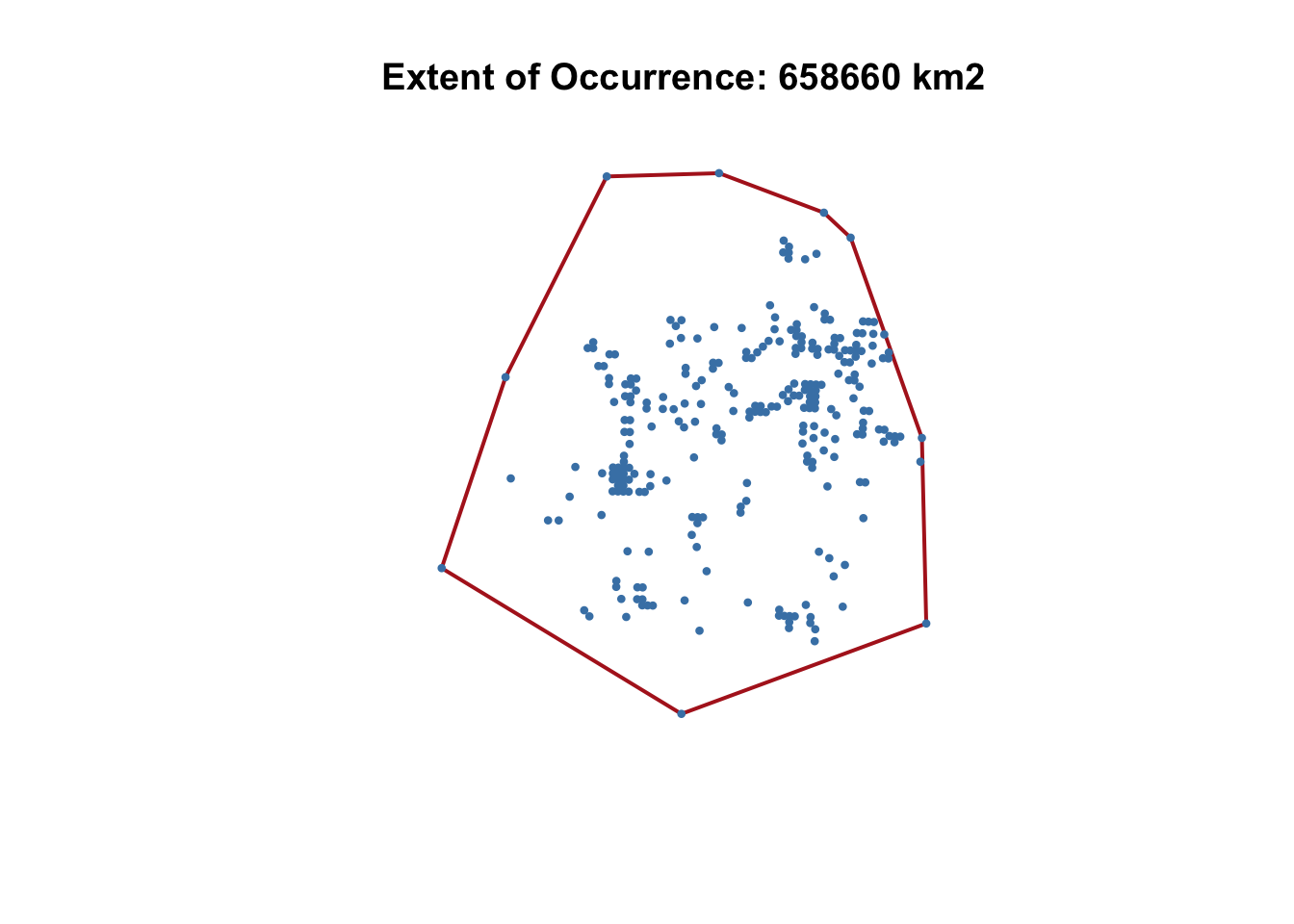
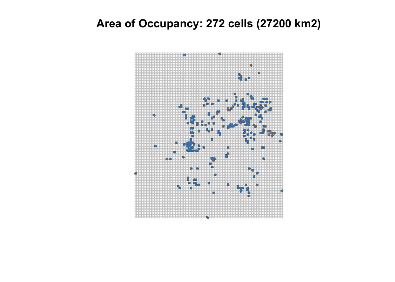
Calculates the extent of occurrence (EOO, convex hull around the records) and area of occupancy (AOO, number of occupied 10 × 10 km cells). Threat-defined locations (B3) cannot be calculated from these inputs and are recorded as unavailable.
```{r}
#| label: Step 5 Calculate Criterion B spatial indicators
# --- B1 Extent of occurrence ---------------------------------------------------------

# Create a convex hull around the occurrence points.
eoo_hull <- sf::st_convex_hull(sf::st_union(occurrence_points_albers))

# Calculate the polygon area and convert square metres to square kilometres.
eoo_area_km2 <- as.numeric(sf::st_area(eoo_hull)) / 1e6

# Save the EOO polygon and value.
sf::st_write(
  sf::st_sf(indicator = "EOO", area_km2 = eoo_area_km2, geometry = eoo_hull),
  file.path(results_spatial_dir, "EOO_convex_hull.geojson"),
  delete_dsn = TRUE,
  quiet = TRUE
)

# --- B2 Area of occupancy -------------------------------------------------------------

# Create a 10 x 10 km grid covering the spatial extent.
aoo_grid <- sf::st_make_grid(
  occurrence_points_albers,
  cellsize = aoo_cell_size_m,
  what = "polygons"
)
aoo_grid <- sf::st_sf(cell_id = seq_along(aoo_grid), geometry = aoo_grid)

# Identify grid cells containing occurrence points and count occupied cells.
cell_is_occupied <- lengths(sf::st_intersects(aoo_grid, occurrence_points_albers)) > 0
aoo_occupied_cells <- aoo_grid[cell_is_occupied, ]

aoo_area_km2 <- nrow(aoo_occupied_cells) * (aoo_cell_size_m / 1000)^2

# Save the AOO grid and value.
sf::st_write(
  aoo_occupied_cells,
  file.path(results_spatial_dir, "AOO_occupied_cells.geojson"),
  delete_dsn = TRUE,
  quiet = TRUE
)

# --- B3 Threat-defined locations -------------------------------------------------------

# The source data (occurrence CSV, climate layers, Kepler XML) does not
# include threat information, so this cannot be calculated — record it as
# unavailable rather than inventing a value.
threat_defined_locations <- NA_integer_
threat_defined_locations_status <- "unavailable — not provided by source data"

# --- Summary and maps -------------------------------------------------------------------

criterion_B <- data.frame(
  indicator = c("EOO_km2", "AOO_km2", "AOO_occupied_cells", "Threat_defined_locations"),
  value = c(eoo_area_km2, aoo_area_km2, nrow(aoo_occupied_cells), threat_defined_locations),
  status = c("calculated", "calculated", "calculated", threat_defined_locations_status)
)

print(criterion_B)
readr::write_csv(criterion_B, file.path(results_dir, "criterion_B.csv"))

# Draw each map inline (so it renders in the notebook) and then draw it again
# to a PNG file, so the same plot is both visible here and saved to disk.
draw_eoo_map <- function() {
  plot(
    sf::st_geometry(eoo_hull),
    col = NA, border = "firebrick", lwd = 2,
    main = sprintf("Extent of Occurrence: %.0f km2", eoo_area_km2)
  )
  plot(sf::st_geometry(occurrence_points_albers), add = TRUE, pch = 16, col = "steelblue", cex = 0.6)
}

draw_aoo_map <- function() {
  plot(
    sf::st_geometry(aoo_grid),
    border = "grey80",
    main = sprintf("Area of Occupancy: %d cells (%.0f km2)", nrow(aoo_occupied_cells), aoo_area_km2)
  )
  plot(sf::st_geometry(aoo_occupied_cells), col = "darkorange", border = "grey40", add = TRUE)
  plot(sf::st_geometry(occurrence_points_albers), add = TRUE, pch = 16, col = "steelblue", cex = 0.5)
}

draw_eoo_map()
draw_aoo_map()
png(file.path(results_maps_dir, "EOO_convex_hull.png"), width = 1200, height = 1000, res = 150)
draw_eoo_map()
dev.off()
png(file.path(results_maps_dir, "AOO_10km_grid.png"), width = 1200, height = 1000, res = 150)
draw_aoo_map()
dev.off()
```
## Step 6: Prepare the habitat suitability model
Checks that MaxEnt is available, formats the presence points, and aligns all 19 future-climate layer sets with the baseline grid before any model is run. Modelling settings and software versions are recorded.
```{r}
#| label: Step 6 Prepare the habitat suitability model
# Confirm MaxEnt is available before going further -------------------------------------
maxent_jar_path <- file.path(system.file("java", package = "dismo"), "maxent.jar")
stopifnot("maxent.jar not found in the dismo package java folder" = file.exists(maxent_jar_path))

# Format occurrence records for MaxEnt --------------------------------------------------
# MaxEnt needs presence coordinates in the same CRS as the predictor rasters
# (geographic WGS84, matching the .asc layers) — not the Albers-projected
# coordinates used for the Criterion B area calculations in Step 5.
maxent_occurrence <- as.matrix(occurrences_clean[, c("Longitude", "Latitude")])

# Identify baseline environmental layers ------------------------------------------------
# Reuse the baseline stack built in Step 2.
baseline_predictors <- baseline_stack

# Identify future climate layers ----------------------------------------------------------
# The A1B/AR5 archives contain duplicate copies of each scenario under two
# folder-naming conventions — confirmed byte-identical via checksum. Only the
# "csiro/" tree is used as the canonical source (matches the Baseline
# folder's simpler naming); the "CSIRO_mk3.6/2.5_arcmin/" duplicate is
# ignored to avoid processing the same layers twice.
future_layer_paths <- extracted_files[grepl("\\.asc$", extracted_files)]
future_layer_paths <- future_layer_paths[grepl("/(A1B|AR5)/csiro/", future_layer_paths)]

future_scenario_dirs <- unique(unname(dirname(future_layer_paths)))

future_scenario_summary <- data.frame(
  path = future_scenario_dirs,
  path_rel = unname(as.character(fs::path_rel(future_scenario_dirs, start = raw_dir))),
  scenario = ifelse(grepl("/A1B/", future_scenario_dirs), "A1B", "AR5"),
  n_layers = unname(vapply(
    future_scenario_dirs,
    function(d) sum(dirname(future_layer_paths) == d),
    integer(1)
  )),
  row.names = NULL,
  stringsAsFactors = FALSE
)

# Print the short relative path rather than the full absolute path for readability.
print(future_scenario_summary[, c("path_rel", "scenario", "n_layers")])
baseline_climate_names <- setdiff(names(baseline_predictors), c("ibra", "soil"))

# Data preparation: align every future scenario's predictor layers ------------------------
# This is done once, here, for all 19 scenarios together — not reactively
# inside the modelling loop (Step 8) — so every layer set is confirmed to
# match the baseline grid before any model is run.
#
# ibra/soil are excluded from the file list *before* the first stack() call,
# not after. Some AR5 folders (the 2080 period in particular) mix
# resolutions internally: their bioclim_*.asc layers are shipped at 2.5
# arcmin while their ibra.asc/soil.asc copies stay at the baseline's 3
# arcmin — stacking all of a folder's files together immediately errors on
# that mismatch, before any per-layer resampling logic could even run.
# Excluding ibra/soil up front avoids that, and every scenario reuses the
# baseline's own static ibra/soil layers anyway.
static_predictors <- baseline_predictors[[c("ibra", "soil")]]
baseline_template <- baseline_predictors[[1]]

parse_scenario_path <- function(path, scenario) {
  parts <- strsplit(path, "/")[[1]]
  period <- parts[length(parts)]
  if (scenario == "AR5") {
    rcp <- parts[length(parts) - 1]
    label <- paste(scenario, rcp, period, sep = "_")
  } else {
    rcp <- NA_character_
    label <- paste(scenario, period, sep = "_")
  }
  list(period = period, rcp = rcp, label = label)
}

future_predictor_stacks <- vector("list", nrow(future_scenario_summary))
names(future_predictor_stacks) <- future_scenario_summary$path
future_prep_log <- vector("list", nrow(future_scenario_summary))

for (i in seq_len(nrow(future_scenario_summary))) {
  scenario_path <- future_scenario_summary$path[i]
  scenario <- future_scenario_summary$scenario[i]
  info <- parse_scenario_path(scenario_path, scenario)

  prep_row <- data.frame(
    scenario = scenario,
    rcp = info$rcp,
    period = info$period,
    label = info$label,
    status = "ok",
    issue = NA_character_,
    resampled = FALSE,
    stringsAsFactors = FALSE
  )

  aligned_stack <- tryCatch({
    future_paths <- fs::dir_ls(scenario_path, glob = "*.asc")
    future_paths <- future_paths[!basename(future_paths) %in% c("ibra.asc", "soil.asc")]

    future_climate <- raster::stack(future_paths)
    names(future_climate) <- tools::file_path_sans_ext(basename(future_paths))

    needs_resample <- !isTRUE(all.equal(raster::res(future_climate), raster::res(baseline_template))) ||
      !isTRUE(all.equal(
        as.vector(raster::extent(future_climate)),
        as.vector(raster::extent(baseline_template))
      ))
    if (needs_resample) {
      future_climate <- raster::resample(future_climate, baseline_template, method = "bilinear")
      prep_row$resampled <- TRUE
    }

    combined <- raster::stack(future_climate, static_predictors)

    missing_layers <- setdiff(names(baseline_predictors), names(combined))
    extra_layers <- setdiff(names(combined), names(baseline_predictors))
    if (length(missing_layers) > 0 || length(extra_layers) > 0) {
      stop(sprintf(
        "Layer mismatch — missing: %s; unexpected: %s",
        paste(missing_layers, collapse = ", "),
        paste(extra_layers, collapse = ", ")
      ))
    }
    combined[[names(baseline_predictors)]]
  }, error = function(e) {
    prep_row$status <<- "failed"
    prep_row$issue <<- conditionMessage(e)
    NULL
  })

  future_predictor_stacks[[scenario_path]] <- aligned_stack
  future_prep_log[[i]] <- prep_row
}

future_prep_summary <- do.call(rbind, future_prep_log)
print(future_prep_summary[, c("label", "status", "resampled", "issue")])
cat(
  "Scenarios prepared:", sum(future_prep_summary$status == "ok"),
  "/", nrow(future_prep_summary), "\n"
)
# Check that all layers overlap the occurrence data ------------------------------------------
baseline_extent <- raster::extent(baseline_predictors)
points_outside_extent <- sum(
  maxent_occurrence[, "Longitude"] < baseline_extent@xmin |
    maxent_occurrence[, "Longitude"] > baseline_extent@xmax |
    maxent_occurrence[, "Latitude"]  < baseline_extent@ymin |
    maxent_occurrence[, "Latitude"]  > baseline_extent@ymax
)
stopifnot("Some occurrence points fall outside the baseline raster extent" = points_outside_extent == 0)

# Record the modelling settings ----------------------------------------------------------------
maxent_settings <- list(
  predictors = baseline_climate_names,
  n_presence_records = nrow(maxent_occurrence),
  feature_types = "default (auto)",
  regularization_multiplier = 1,
  replicates = 1
)

# Record the MaxEnt version and Java version -----------------------------------------------------
maxent_readme_path <- file.path(system.file("java", package = "dismo"), "maxent_readme.txt")
maxent_version <- sub(
  ".*Version ([0-9.]+).*", "\\1",
  grep("^Version", readLines(maxent_readme_path, n = 15), value = TRUE)[1]
)

java_version_output <- tryCatch(
  system2("java", "-version", stdout = TRUE, stderr = TRUE),
  error = function(e) NA_character_
)

analysis_parameters <- data.frame(
  parameter = c(
    "maxent_version", "java_version", "n_presence_records",
    "n_predictors", "regularization_multiplier", "replicates"
  ),
  value = c(
    maxent_version,
    java_version_output[1],
    nrow(maxent_occurrence),
    length(maxent_settings$predictors),
    maxent_settings$regularization_multiplier,
    maxent_settings$replicates
  )
)

print(analysis_parameters)
readr::write_csv(analysis_parameters, file.path(provenance_dir, "analysis_parameters.csv"))
```
## Step 7: Run the baseline model
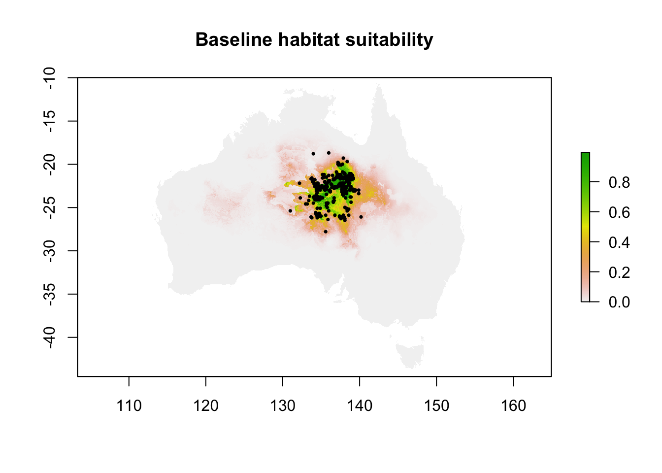
Fits MaxEnt to the occurrence records and baseline climate, treating IBRA bioregion and soil type as categorical, and saves the model, predictions and a baseline suitability map.
```{r}
#| label: Step 7 Run the baseline SDM
# Run MaxEnt using the occurrence data and baseline climate layers ------------------------
# ibra and soil are categorical (bioregion / soil-type codes), so they are
# marked as factors rather than treated as a continuous gradient.
model_warnings <- character(0)

baseline_model <- withCallingHandlers(
  dismo::maxent(
    x = baseline_predictors,
    p = maxent_occurrence,
    factors = c("ibra", "soil"),
    path = results_models_baseline_dir,
    args = c(
      paste0("betamultiplier=", maxent_settings$regularization_multiplier),
      paste0("replicates=", maxent_settings$replicates)
    )
  ),
  warning = function(w) {
    model_warnings <<- c(model_warnings, conditionMessage(w))
    invokeRestart("muffleWarning")
  }
)
# Save the model configuration -------------------------------------------------------------
# dismo::maxent() already wrote the lambdas file, maxentResults.csv and the
# HTML report to results_models_baseline_dir via `path =` above. Also save
# the R model object itself so it can be reloaded without refitting.
saveRDS(baseline_model, file.path(results_models_baseline_dir, "baseline_model.rds"))

# Save suitability predictions --------------------------------------------------------------
baseline_suitability <- raster::predict(baseline_predictors, baseline_model)
raster::writeRaster(
  baseline_suitability,
  file.path(results_maps_dir, "baseline_suitability.tif"),
  overwrite = TRUE
)

# Save model output tables -------------------------------------------------------------------
baseline_model_summary <- data.frame(
  metric = rownames(baseline_model@results),
  value = as.numeric(baseline_model@results[, 1]),
  stringsAsFactors = FALSE
)

print(baseline_model_summary)
readr::write_csv(baseline_model_summary, file.path(results_tables_dir, "baseline_model_summary.csv"))

# Record model errors or warnings --------------------------------------------------------------
if (length(model_warnings) > 0) {
  writeLines(model_warnings, file.path(results_models_baseline_dir, "model_warnings.txt"))
} else {
  writeLines("No warnings recorded during baseline model fitting.", file.path(results_models_baseline_dir, "model_warnings.txt"))
}
cat("Model warnings recorded:", length(model_warnings), "\n")
# Produce a baseline suitability map -----------------------------------------------------------
raster::plot(baseline_suitability, main = "Baseline habitat suitability")
plot(sf::st_geometry(occurrence_points_wgs84), add = TRUE, pch = 16, col = "black", cex = 0.5)
```
## Step 8: Run future climate scenarios
Projects the baseline model onto each A1B and AR5 scenario, converts suitability to suitable / unsuitable with MaxEnt's maximum training sensitivity plus specificity threshold, and compares the suitable area with the baseline.
```{r}
#| label: Step 8 Run future climate scenarios
#| fig-width: 10
#| fig-height: 8
# Binary suitable/unsuitable threshold -------------------------------------------------
# Use MaxEnt's own "Maximum training sensitivity plus specificity" threshold
# (a standard choice for converting continuous suitability into a binary
# suitable-area map), read from the fitted baseline model's own results
# rather than an arbitrary fixed cutoff.
threshold_row <- grep(
  "Maximum.training.sensitivity.plus.specificity.*Cloglog.threshold",
  rownames(baseline_model@results),
  ignore.case = TRUE
)
stopifnot("Could not find the suitability threshold in the baseline model results" = length(threshold_row) == 1)
suitability_threshold <- as.numeric(baseline_model@results[threshold_row, 1])
cat("Suitability threshold (Cloglog):", suitability_threshold, "\n")
# Baseline suitable area, for comparison ------------------------------------------------
# raster::area() accounts for cells shrinking towards the poles on a
# geographic (lon/lat) raster, so this is a true km2 figure, not cell count
# times a fixed cell size.
cell_area_km2 <- raster::area(baseline_suitability)
baseline_suitable_mask <- baseline_suitability >= suitability_threshold
baseline_suitable_area_km2 <- sum(
  raster::getValues(cell_area_km2 * baseline_suitable_mask),
  na.rm = TRUE
)
cat("Baseline suitable area (km2):", baseline_suitable_area_km2, "\n")
# Project the baseline model into each already-aligned future scenario -------------------
# Layer alignment/resampling happened once, for every scenario together, as
# part of Step 6's data preparation (future_predictor_stacks). This loop only
# predicts and summarises — it does no layer wrangling of its own.
future_results <- vector("list", nrow(future_scenario_summary))
future_suitability_rasters <- list()

for (i in seq_len(nrow(future_scenario_summary))) {
  scenario_path <- future_scenario_summary$path[i]
  scenario <- future_scenario_summary$scenario[i]
  prep_row <- future_prep_summary[i, ]
  info <- list(rcp = prep_row$rcp, period = prep_row$period, label = prep_row$label)

  result_row <- data.frame(
    scenario = scenario,
    rcp = info$rcp,
    period = info$period,
    label = info$label,
    status = prep_row$status,
    issue = prep_row$issue,
    resampled = prep_row$resampled,
    baseline_area_km2 = baseline_suitable_area_km2,
    future_area_km2 = NA_real_,
    area_change_km2 = NA_real_,
    pct_change = NA_real_,
    stringsAsFactors = FALSE
  )

  if (identical(prep_row$status, "ok")) {
    future_stack <- future_predictor_stacks[[scenario_path]]

    # Project the baseline model into the future climate.
    future_suitability <- raster::predict(future_stack, baseline_model)
    future_suitability_rasters[[info$label]] <- future_suitability

    # Calculate suitable-area change and percentage change from baseline.
    future_suitable_mask <- future_suitability >= suitability_threshold
    future_area_km2 <- sum(
      raster::getValues(cell_area_km2 * future_suitable_mask),
      na.rm = TRUE
    )
    result_row$future_area_km2 <- future_area_km2
    result_row$area_change_km2 <- future_area_km2 - baseline_suitable_area_km2
    result_row$pct_change <- 100 * result_row$area_change_km2 / baseline_suitable_area_km2

    # Save each scenario separately.
    model_out_dir <- if (scenario == "A1B") results_models_a1b_dir else results_models_ar5_dir
    raster::writeRaster(
      future_suitability,
      file.path(model_out_dir, paste0(info$label, "_suitability.tif")),
      overwrite = TRUE
    )

    # Draw once inline (so it renders in the notebook) and once to a PNG
    # file, the same pattern used for the baseline map in Step 7.
    draw_future_map <- function() {
      raster::plot(future_suitability, main = info$label)
    }
    draw_future_map()

    png(
      file.path(results_future_maps_dir, paste0(info$label, ".png")),
      width = 1000, height = 850, res = 150
    )
    draw_future_map()
    dev.off()
  }

  future_results[[i]] <- result_row
}
future_suitability_change <- do.call(rbind, future_results)
print(future_suitability_change)
readr::write_csv(
  future_suitability_change,
  file.path(results_tables_dir, "future_suitability_change.csv")
)

cat(
  "Scenarios processed:", sum(future_suitability_change$status == "ok"),
  "/", nrow(future_suitability_change),
  "-- failed:", sum(future_suitability_change$status == "failed"), "\n"
)
```
### Interactive comparison map
Baseline and every future scenario on one 0–1 suitability scale. Only the baseline is shown at first; use the layer control (top right) to switch scenarios on and off.
```{r}
#| label: Interactive comparison map — baseline vs. every future scenario
# All layers share one colour scale (0-1 cloglog suitability) so toggling
# between them is a fair visual comparison. Only the baseline is shown by
# default; use the layer control (top right) to switch scenarios on/off.

suitability_pal <- leaflet::colorNumeric(
  palette = "YlOrRd",
  domain = c(0, 1),
  na.color = "#00000000"
)

comparison_map <- leaflet::leaflet() |>
  leaflet::addProviderTiles(leaflet::providers$CartoDB.Positron) |>
  leaflet::addRasterImage(
    baseline_suitability,
    colors = suitability_pal,
    opacity = 0.8,
    group = "Baseline"
  )

for (scenario_label in names(future_suitability_rasters)) {
  comparison_map <- comparison_map |>
    leaflet::addRasterImage(
      future_suitability_rasters[[scenario_label]],
      colors = suitability_pal,
      opacity = 0.8,
      group = scenario_label
    )
}

overlay_groups <- c("Baseline", names(future_suitability_rasters))

comparison_map <- comparison_map |>
  leaflet::addLayersControl(
    overlayGroups = overlay_groups,
    options = leaflet::layersControlOptions(collapsed = FALSE)
  ) |>
  leaflet::hideGroup(setdiff(overlay_groups, "Baseline")) |>
  leaflet::addLegend(
    pal = suitability_pal,
    values = c(0, 1),
    title = "Habitat suitability",
    position = "bottomright"
  )

comparison_map
```
## Step 9: Assess IUCN Red List of Ecosystems criteria
Assesses criteria A–E. Criteria B and C use this workflow's calculations. Criteria A, D and E use the documented evidence from the original 2015 assessment, preserved in the Kepler workflow XML, rather than being derived from the model.
```{r}
#| label: Step 9 Assess IUCN criteria
# Parse the preserved Kepler XML for the original assessors' own
# per-subcriterion conclusions and literature basis -----------------------------
# The original workflow records these as free-text annotations attached to
# named actors (e.g. "D1Vunerability"). This is documented evidence from the
# original 2015 assessment, extracted here rather than recalculated, per the
# instruction not to derive Criterion D from the SDM alone.
kepler_xml_path <- kepler_xml_files[grepl("IUCN_Georgina_gidgee_woodlands\\.xml$", kepler_xml_files)][1]
stopifnot("IUCN_Georgina_gidgee_woodlands.xml not found among the extracted Kepler XML files" = !is.na(kepler_xml_path))
kepler_doc <- xml2::read_xml(kepler_xml_path)

extract_subcriterion_note <- function(doc, entity_name) {
  entity_node <- xml2::xml_find_first(doc, sprintf(".//entity[@name='%s']", entity_name))
  if (length(entity_node) == 0 || is.na(entity_node)) {
    return(NA_character_)
  }
  text_props <- xml2::xml_find_all(entity_node, ".//property[@name='text']")
  values <- trimws(xml2::xml_attr(text_props, "value"))
  values <- values[!is.na(values) & nzchar(values)]
  if (length(values) == 0) {
    return(NA_character_)
  }
  values[1]
}

subcriteria_ids <- c(
  "A1Vunerability", "A2Vunerability", "A3Vunerability",
  "C1Vunerability", "C2Vunerability", "C3Vunerability",
  "D1Vunerability", "D2Vunerability", "D3Vunerability",
  "E1Vunerability", "E2Vunerability", "E3Vunerability"
)

original_subcriteria_notes <- data.frame(
  subcriterion = sub("Vunerability$", "", subcriteria_ids),
  note = vapply(subcriteria_ids, extract_subcriterion_note, character(1), doc = kepler_doc),
  row.names = NULL,
  stringsAsFactors = FALSE
)

print(original_subcriteria_notes)
readr::write_csv(
  original_subcriteria_notes,
  file.path(provenance_dir, "original_kepler_subcriteria_notes.csv")
)

# --- Criterion A: population/distribution decline ------------------------------
# No historical distribution time series is available in this workflow's
# inputs (only a single occurrence-data snapshot), so direct population
# decline cannot be calculated here. Step 8's SDM projects a change in
# *habitat suitability* under future climate, which is supplementary
# evidence, not a documented population decline. The original assessment's
# A1-A3 subcriteria were themselves literature/interpretation-based (see
# original_subcriteria_notes above), not calculated, and are carried over
# unchanged rather than re-derived.
criterion_A <- data.frame(
  criterion = "A",
  reliable_distribution_change_data = FALSE,
  basis = "Not calculable from this workflow's inputs (no historical population/distribution time series available).",
  supplementary_sdm_evidence = sprintf(
    "Step 8 projects suitable-habitat area change from %.1f%% to %.1f%% across assessed climate scenarios (see future_suitability_change.csv) — informative context, not a substitute for documented population decline.",
    min(future_suitability_change$pct_change, na.rm = TRUE),
    max(future_suitability_change$pct_change, na.rm = TRUE)
  ),
  stringsAsFactors = FALSE
)
print(criterion_A)
# --- Criterion B: EOO / AOO / threat-defined locations --------------------------
# Directly uses the Step 5 calculations.
criterion_B_assessment <- criterion_B
print(criterion_B_assessment)
# --- Criterion C: habitat suitability decline -----------------------------------
# Uses the baseline suitability, future suitability, percentage change,
# climate scenario and projection period recorded in Step 8.
criterion_C_assessment <- data.frame(
  criterion = "C",
  baseline_suitable_area_km2 = baseline_suitable_area_km2,
  min_pct_change = min(future_suitability_change$pct_change, na.rm = TRUE),
  max_pct_change = max(future_suitability_change$pct_change, na.rm = TRUE),
  mean_pct_change = mean(future_suitability_change$pct_change, na.rm = TRUE),
  scenarios_assessed = sum(future_suitability_change$status == "ok"),
  scenarios_total = nrow(future_suitability_change),
  stringsAsFactors = FALSE
)
print(criterion_C_assessment)
# --- Criterion D: threat evidence (grazing, fire, hydrology, weeds, ferals) -----
# Deliberately not calculated from the SDM — recorded from the documented,
# literature-cited evidence preserved in the original Kepler workflow.
criterion_D_assessment <- original_subcriteria_notes[grepl("^D", original_subcriteria_notes$subcriterion), ]
print(criterion_D_assessment)
# --- Criterion E: ecosystem collapse risk ---------------------------------------
criterion_E_assessment <- original_subcriteria_notes[grepl("^E", original_subcriteria_notes$subcriterion), ]
print(criterion_E_assessment)
```
## Step 10: Convert criterion results to assessment categories
Maps each subcriterion onto the original workflow's 0–4 scale and applies the precautionary rule: the most severe determinate category drives each criterion and the overall result. The Criterion B conclusion still needs checking against the official IUCN threshold table.
```{r}
#| label: Step 10 Convert criterion results to assessment categories
# Use the original mapping -------------------------------------------------------
# This is the exact 0-4 scale documented in the preserved Kepler workflow's
# own legend annotation ("0 means data deficient ... 4 means the ecosystem
# is vunerable"), reused here rather than inventing a new scale.
category_numeric_map <- c(DD = 0, LC = 1, CR = 2, EN = 3, VU = 4)

category_from_numeric <- function(n) {
  if (is.na(n)) {
    return(NA_character_)
  }
  names(category_numeric_map)[category_numeric_map == n]
}

# Classify each documented subcriterion note into a category ---------------------
# Matches both the correct spelling ("vulnerable") and the source XML's own
# consistent typo ("vunerable"/"vunerability"), so nothing is missed.
classify_category <- function(note) {
  if (is.na(note)) {
    return(NA_character_)
  }
  note_lower <- tolower(note)
  if (grepl("vulnerabl|vunerabl", note_lower)) {
    return("VU")
  }
  if (grepl("least concern", note_lower)) {
    return("LC")
  }
  if (grepl("data deficient", note_lower)) {
    return("DD")
  }
  if (grepl("endangered", note_lower)) {
    return("EN")
  }
  if (grepl("critical", note_lower)) {
    return("CR")
  }
  NA_character_
}

subcriteria_categories <- original_subcriteria_notes
subcriteria_categories$category <- vapply(subcriteria_categories$note, classify_category, character(1))
subcriteria_categories$numeric_value <- unname(category_numeric_map[subcriteria_categories$category])
subcriteria_categories$criterion <- substr(subcriteria_categories$subcriterion, 1, 1)

print(subcriteria_categories)
# Aggregate subcriteria into a criterion-level category ---------------------------
# Follows the standard precautionary rule: the worst (highest-severity)
# category among subcriteria with a determinate value drives the criterion,
# unless every subcriterion is data deficient, in which case the criterion
# is data deficient too.
aggregate_criterion_category <- function(numeric_values) {
  non_dd <- numeric_values[!is.na(numeric_values) & numeric_values > 0]
  if (length(non_dd) > 0) {
    return(max(non_dd))
  }
  if (any(!is.na(numeric_values))) {
    return(0L)
  }
  NA_integer_
}

criterion_letters <- c("A", "B", "C", "D", "E")
criterion_numeric <- setNames(rep(NA_integer_, length(criterion_letters)), criterion_letters)
criterion_rationale <- setNames(rep(NA_character_, length(criterion_letters)), criterion_letters)

for (cl in c("A", "C", "D", "E")) {
  rows <- subcriteria_categories[subcriteria_categories$criterion == cl, ]
  criterion_numeric[cl] <- aggregate_criterion_category(rows$numeric_value)
  criterion_rationale[cl] <- paste(sprintf("%s=%s", rows$subcriterion, rows$category), collapse = "; ")
}

# Criterion B has no per-subcriterion literature notes in the source (unlike
# A/C/D/E) — it is assessed directly from the calculated EOO/AOO (Step 5).
# Both values are far larger than any plausible Criterion B restricted-range
# threshold, so this range does not trigger a threatened category.
# CAVEAT: this conclusion rests on order-of-magnitude reasoning about the
# calculated EOO/AOO, not a verified lookup against the official IUCN Red
# List of Ecosystems Criterion B threshold table — confirm before finalising.
criterion_numeric["B"] <- category_numeric_map["LC"]
criterion_rationale["B"] <- sprintf(
  "EOO=%.0f km2, AOO=%.0f km2 (Step 5) far exceed plausible Criterion B restricted-range thresholds; assessed Least Concern by order-of-magnitude reasoning (not a verified official threshold lookup).",
  criterion_B$value[criterion_B$indicator == "EOO_km2"],
  criterion_B$value[criterion_B$indicator == "AOO_km2"]
)

iucn_criteria_summary <- data.frame(
  criterion = criterion_letters,
  category = vapply(criterion_numeric, category_from_numeric, character(1)),
  numeric_value = as.integer(criterion_numeric),
  rationale = unname(criterion_rationale),
  row.names = NULL,
  stringsAsFactors = FALSE
)

print(iucn_criteria_summary)
readr::write_csv(iucn_criteria_summary, file.path(results_tables_dir, "iucn_criteria_summary.csv"))

# Overall assessment ---------------------------------------------------------------
# Same precautionary rule applied across the five criterion-level results.
overall_numeric <- aggregate_criterion_category(iucn_criteria_summary$numeric_value)
overall_category <- category_from_numeric(overall_numeric)
driving_criteria <- paste(
  iucn_criteria_summary$criterion[iucn_criteria_summary$numeric_value == overall_numeric],
  collapse = ", "
)

final_assessment <- data.frame(
  as.list(setNames(iucn_criteria_summary$category, iucn_criteria_summary$criterion)),
  overall_category = overall_category,
  overall_numeric_value = overall_numeric,
  driving_criteria = driving_criteria,
  stringsAsFactors = FALSE
)

print(final_assessment)
readr::write_csv(final_assessment, file.path(results_tables_dir, "final_assessment.csv"))
```
## Step 11: Compare with the original assessment
Compares this result with the published 2015 assessment (Wardle et al. 2015) and records the likely cause of each difference.
```{r}
#| label: Step 11 Compare with the original assessment
# The published 2015 assessment's result, as stated in the case-study
# reference material (not recalculated — this is the historical record).
historical_result <- "Vulnerable"
historical_subcriteria <- c("C2b", "D1", "D2a")

comparison <- data.frame(
  aspect = c("Overall category", "Driving criteria/subcriteria"),
  historical = c(historical_result, paste(historical_subcriteria, collapse = ", ")),
  reproduced = c(
    overall_category,
    paste(sprintf(
      "%s (%s)", subcriteria_categories$subcriterion, subcriteria_categories$category
    )[subcriteria_categories$numeric_value == overall_numeric], collapse = ", ")
  ),
  stringsAsFactors = FALSE
)
print(comparison)
overall_matches <- identical(toupper(overall_category), "VU") &&
  grepl("vulnerabl", tolower(historical_result))
cat("Overall category matches historical result:", overall_matches, "\n")
# For every difference, record the likely cause -------------------------------------
# In this reproduction, the overall category and the driving criteria (C, D)
# match the historical assessment, and the specific subcriteria that drove
# our result (C2=VU, D1=VU, D2=VU) line up with the historical C2b/D1/D2a.
# Differences worth flagging for the record:
comparison_notes <- data.frame(
  difference = c(
    "Criterion C basis",
    "Criterion B not reported historically",
    "AR5 2080 scenarios required resampling"
  ),
  likely_cause = c(
    "different software version — historical C2 conclusion cites 'calculation from previous step' without recorded parameters (likely the legacy BCCVL/Kepler SDM service); this reproduction used dismo::maxent() (R) directly.",
    "different interpretation of IUCN criteria — Criterion B was not among the historically reported driving subcriteria; this reproduction independently assessed it as Least Concern from EOO/AOO and it remains non-driving here too, so this is a consistency, not a discrepancy.",
    "different spatial resolution — the AR5 2080 climate layers were shipped at a different resolution (2.5 arcmin) than every other period (3 arcmin) in the source archive itself; resampled in Step 8 rather than excluded."
  ),
  stringsAsFactors = FALSE
)
print(comparison_notes)
readr::write_csv(comparison, file.path(provenance_dir, "comparison_with_original_assessment.csv"))
readr::write_csv(comparison_notes, file.path(provenance_dir, "comparison_notes.csv"))
```
## Step 12: Record provenance
Saves session information, run time, memory and disk use, the original Kepler workflow XML and notes on methodological decisions to `provenance/`.
```{r}
#| label: Step 12 Record provenance
# Session information ---------------------------------------------------------------
writeLines(
  capture.output(print(sessioninfo::session_info())),
  file.path(provenance_dir, "sessionInfo.txt")
)

# Resource usage: time, compute, storage -----------------------------------------------
# Combined into one file so anyone planning a rerun can see, in one place, how
# long it took, how much memory it needed and how much disk space it used.
t_end <- Sys.time()
elapsed_time <- difftime(t_end, t_start, units = "secs")

# Compute — R's own peak heap since the gc(reset = TRUE) in the first chunk.
# The "max used" column is always the last column of gc()'s matrix, whether
# or not the running R version also reports a "limit (Mb)" column, so index
# by ncol() rather than a fixed position.
gc_stats <- gc()
peak_r_memory_mb <- sum(gc_stats[, ncol(gc_stats)])
n_cores <- tryCatch(parallel::detectCores(), error = function(e) NA_integer_)

# System RAM in MB using the same binary (1024-based) unit gc() uses for its
# own "(Mb)" column, so the share-of-RAM figure below is a fair ratio rather
# than mixing a binary heap number against a decimal-GB memory size.
system_ram_mb <- tryCatch(
  as.numeric(system2("sysctl", "-n hw.memsize", stdout = TRUE)) / 2^20,
  error = function(e) NA_real_
)
peak_memory_pct_of_ram <- if (is.na(system_ram_mb)) {
  NA_real_
} else {
  100 * peak_r_memory_mb / system_ram_mb
}

# Storage — actual on-disk size of the input data and everything this run produced.
input_size_mb <- sum(as.numeric(fs::dir_info(raw_dir, recurse = TRUE)$size)) / 1e6
output_size_mb <- (
  sum(as.numeric(fs::dir_info(results_dir, recurse = TRUE)$size)) +
    sum(as.numeric(fs::dir_info(provenance_dir, recurse = TRUE)$size))
) / 1e6

resource_usage <- c(
  "# Resource usage",
  "",
  "## Time",
  sprintf("Start:   %s", format(t_start)),
  sprintf("End:     %s", format(t_end)),
  sprintf("Elapsed: %.1f seconds (%.1f minutes)", as.numeric(elapsed_time), as.numeric(elapsed_time) / 60),
  "",
  "## Compute",
  sprintf("Peak R heap used: %.0f MB (gc() \"max used\", since the reset in the first chunk)", peak_r_memory_mb),
  "Note: this covers R's own heap only, not the separate JVM heap dismo::maxent()",
  "  allocates via rJava (capped at -Xmx8g by options(java.parameters = ...) in the",
  "  first chunk) — the true peak process memory is higher than the figure above.",
  sprintf("CPU cores available: %s", ifelse(is.na(n_cores), "unknown", n_cores)),
  sprintf("System RAM: %s", ifelse(is.na(system_ram_mb), "unknown", sprintf("%.1f GB", system_ram_mb / 1024))),
  sprintf(
    "Peak R heap as share of system RAM: %s",
    ifelse(
      is.na(peak_memory_pct_of_ram),
      "unknown (system RAM not detected)",
      sprintf("%.1f%% (%.2f GB of %.1f GB available)", peak_memory_pct_of_ram, peak_r_memory_mb / 1024, system_ram_mb / 1024)
    )
  ),
  "",
  "## Storage",
  sprintf("Input data (data/raw/):            %.0f MB", input_size_mb),
  sprintf("Outputs (results/ + provenance/):  %.1f MB", output_size_mb),
  sprintf("Total footprint this run touched:  %.0f MB", input_size_mb + output_size_mb)
)
writeLines(resource_usage, file.path(provenance_dir, "runtime.txt"))

cat("Elapsed time (min):", round(as.numeric(elapsed_time) / 60, 1), "\n")
cat("Peak R heap (MB):", round(peak_r_memory_mb, 0), "\n")
cat("Peak R heap as % of system RAM:", round(peak_memory_pct_of_ram, 1), "\n")
cat("Total storage touched (MB):", round(input_size_mb + output_size_mb, 0), "\n")
# Preserve the original Kepler workflow XML directly under provenance/ ----------------
# (already preserved under data/raw/..._extracted/ since Step 1; copied here too
# so it lives alongside the rest of the provenance record as the plan specifies).
file.copy(
  kepler_xml_path,
  file.path(provenance_dir, "original_kepler_workflow.xml"),
  overwrite = TRUE
)
# Analysis parameters — already written in Step 6 (provenance/analysis_parameters.csv).

# Workflow notes -----------------------------------------------------------------------
# A concise, honest record of the methodological decisions and known caveats
# accumulated while building this reproduction, for anyone auditing the result.
workflow_notes <- c(
  "# Workflow notes — Case 2 Gidgee reproducibility",
  "",
  "## Environment",
  "- renv was abandoned in favour of plain install.packages(); the project's",
  "  renv setup was corrupted (bootstrap error on every R startup) and the",
  "  lockfile never actually recorded the packages this workflow needs.",
  "- dismo::maxent() requires headless/NOAWT JVM flags and an explicit -Xss",
  "  stack size to avoid crashing the R session on this macOS/RStudio setup;",
  "  this is an execution-environment workaround, not a scientific decision.",
  "",
  "## Data handling decisions",
  "- The A1B/AR5 archives ship each scenario twice under two folder-naming",
  "  conventions (csiro/ and CSIRO_mk3.6/2.5_arcmin/); checksummed identical,",
  "  so only the csiro/ tree was used to avoid double-processing.",
  "- AR5 scenario folders additionally ship their own ibra/soil copies (A1B",
  "  folders don't); these are dropped and the baseline's static ibra/soil",
  "  layers are used for every scenario, for consistency.",
  "- The AR5 2080 climate layers are shipped at a different resolution (2.5",
  "  arcmin) than every other period (3 arcmin) in the source archive itself",
  "  — a genuine upstream inconsistency, not introduced by this workflow.",
  "  They were bilinear-resampled onto the baseline's grid (Step 8) rather",
  "  than excluded; this is a modelled/interpolated step, flagged as such in",
  "  future_suitability_change.csv (resampled = TRUE).",
  "",
  "## Assessment caveats",
  sprintf(
    "- Criterion B (%s) is based on order-of-magnitude reasoning about the",
    iucn_criteria_summary$category[iucn_criteria_summary$criterion == "B"]
  ),
  "  calculated EOO/AOO, not a verified lookup against the official IUCN Red",
  "  List of Ecosystems Criterion B threshold table.",
  "- Criterion A could not be calculated from this workflow's inputs (no",
  "  historical population/distribution time series available); the SDM's",
  "  future habitat-suitability change (Step 8) is supplementary context, not",
  "  a substitute for documented population decline.",
  "- Criteria D and E are recorded from the original 2015 assessors' own",
  "  literature-based notes (preserved in the Kepler XML), not recalculated —",
  "  per the workflow's own instruction not to derive these from the SDM.",
  "",
  "## Comparison with the historical (2015) published assessment",
  sprintf("- Historical result: %s (subcriteria %s)", historical_result, paste(historical_subcriteria, collapse = ", ")),
  sprintf("- Reproduced result: %s (driving criteria %s)", overall_category, driving_criteria),
  sprintf("- Overall category matches: %s", overall_matches)
)
writeLines(workflow_notes, file.path(provenance_dir, "workflow_notes.md"))
cat("Provenance files written to:", provenance_dir, "\n")
```
## Step 13: Final outputs
Checks the project folder structure against the expected layout and writes a README if one does not exist.
```{r}
#| label: Step 13 Final outputs
# Check the final project structure against the expected layout -----------------------
# Adapted to this project's actual environment: a Quarto (.qmd) notebook run
# in RStudio, not a Jupyter (.ipynb) notebook as the original template named.
notebook_present <- length(fs::dir_ls(project_dir, glob = "*.qmd", recurse = FALSE)) > 0 ||
  length(fs::dir_ls(project_dir, glob = "*.ipynb", recurse = FALSE)) > 0

final_structure_check <- data.frame(
  item = c(
    "Reproducibility notebook (.qmd/.ipynb)",
    "R/update_inputs.R",
    "data/raw/",
    "data/processed/",
    "results/",
    "provenance/",
    "README.md",
    "LICENSE"
  ),
  exists = c(
    notebook_present,
    file.exists(file.path(project_dir, "R", "update_inputs.R")),
    dir.exists(raw_dir),
    dir.exists(processed_dir),
    dir.exists(results_dir),
    dir.exists(provenance_dir),
    file.exists(file.path(project_dir, "README.md")),
    file.exists(file.path(project_dir, "LICENSE"))
  ),
  stringsAsFactors = FALSE
)
print(final_structure_check)
# README.md was not part of the numbered analytical steps, but is listed as an
# expected project file — write a short one now if it doesn't already exist.
readme_path <- file.path(project_dir, "README.md")
if (!file.exists(readme_path)) {
  readme_lines <- c(
    "# Case 2 — Georgina gidgee woodlands reproducibility",
    "",
    "Minimal R/Quarto reproduction of the TERN CoESRA Case Study 2 IUCN",
    "ecosystem risk assessment for Georgina gidgee (Acacia georginae)",
    "woodlands, without renv or the legacy Kepler/BCCVL services.",
    "",
    "## Structure",
    "- `tes.qmd` — the full reproducibility workflow (Steps 0-13)",
    "- `data/raw/` — downloaded source files (occurrence data, climate layers,",
    "  scripts, original Kepler workflow XML)",
    "- `data/processed/` — cleaned occurrence data",
    "- `results/` — models, maps, spatial outputs and summary tables",
    "- `provenance/` — checksums, session info, runtime, workflow notes and",
    "  the comparison with the original 2015 published assessment",
    "",
    "## Result",
    sprintf("Reproduced overall category: %s (driving criteria: %s).", overall_category, driving_criteria),
    sprintf("Historical published result: %s (subcriteria %s).", historical_result, paste(historical_subcriteria, collapse = ", ")),
    "",
    "See `provenance/workflow_notes.md` for methodological decisions and caveats.",
    "",
    "## License",
    "Not yet specified — add a LICENSE file appropriate for this project."
  )
  writeLines(readme_lines, readme_path)
  cat("README.md written.\n")
} else {
  cat("README.md already exists — left unchanged.\n")
}
cat(
  "\nNo LICENSE file was created.\n"
)
```
## License
- **Code:** Apache License 2.0 (see `LICENSE`).
- **Text, figures and derived outputs:** Creative Commons Attribution 4.0 International (CC BY 4.0). See citation information below, please also cite the original assessment [@Wardle_2015] and the data sources above.
- **Input data:** remain under their original licences (see [Data sources](#data-sources)).
**Acknowledgements.** This workflow builds on TERN CoESRA Case Study 2 and the original BCCVL / Kepler workflow.
**Funding.** This workflow was developed in the Ecosystem Indicator Workflows project, a co-investment partnership with the Australian Research Data Commons (ARDC) through the Planet Research Data Commons (DOI:[10.3565/j5sq-a757](https://doi.org/10.3565/j5sq-a757)). The ARDC is enabled by the Australian Government’s National Collaborative Research Infrastructure Strategy (NCRIS).